Frequently Asked Questions
- Details
-
Last Updated: Wednesday, 21 August 2013 11:44
General
Input parameters
Topologies
Problems
General
-
If I would like to visit Groningen to learn how to use MARTINI should I be worried about the weather?
Don't worry, the weather is fine.
-
Is there financial support for a visit to Groningen?
Your best option is to try to get an HPC-Europa Transnational Access grant. Transnational Access is an inter-disciplinary research visit programme. It enables researchers working in any eligible country in Europe to visit a participating research institute to carry out a collaborative visit of up to 3 months´ duration, and to gain access to some of the most powerful High Performance Computing (HPC) facilities in Europe. Researchers may visit any institute associated with a number of HPC centres including SARA in the Netherlands. Our institute is associated with SARA so the HPC grant allows you to stay in our group long enough to learn the do's and don'ts of Martini. We hosted already some ten students through this program over the past five years. For details how to apply, see the website http://www.hpc-europa.eu/
Martini is the nickname of the city of Groningen where the forcefield was developed. It also reflects the universality of the cocktail with the same name; how a few simple ingredients (chemical building blocks) can be endlessly varied to create a complex palette of taste.
However, it is also an acronym for:
° MARrink's Toolkit INItiative
° Maybe A Realistic Theory to Investigate N-body Interactions
Please help me find the ultimate acronym ..

Martinitoren ( Martini tower) in Groningen
-
Can I use Martini to study protein folding?
No, at the moment the secondary structure is an input parameter of the model, which implies that secondary structure elements remain fixed during the simulation. Tertiary structural changes, however, are allowed and in principle realistically described with Martini.
-
How should I interpret the time scale?
The Martini dynamics is faster than the all-atom dynamics because the coarse-grained interactions are much smoother compared to atomistic interactions. The effective friction caused by the fine grained degrees of freedom is missing. Based on comparison of diffusion constants in the Martini model and in atomistic models, the effective time sampled using CG interactions is 3-8 fold larger. When interpreting the simulation results with the Martini model, we use a standard conversion factor of 4, which is the effective speed-up factor in the diffusion dynamics of Martini water compared to real water. The same order of acceleration of the overall dynamics is also observed for a number of other processes, including the permeation rate of water across a membrane, the sampling of the local configurational space of a lipid, and the aggregation rate of lipids into bilayers or vesicles. However, the speed-up factor might be quite different in other systems or for other processes. Particularly for protein systems no extensive testing of the actual speed up due to the caorse-grained dynamics has been performed, although protein translational and rotational diffusion was found to be in good agreement with experimental data in simulations of rhodopsin. In general, however, the time scale of the Martini simulations has to be interpreted with care.
-
How to reintroduce atomistic detail into Martini?
For this you can use our Reverse Transformation Tool explained on the tutorial page.
-
Can I do multiscale simulations with Martini?
We developed a method to do hybrid simulations using virual sites, as described in [1], but so far it works well only for relatively simple systems (e.g. butane). We are working on it ...
[1] A.J. Rzepiela, M. Louhivuori, C. Peter, S.J. Marrink. Hybrid simulations: combining atomistic and coarse-grained force fields using virtual sites. Phys. Chem. Chem. Phys., 13:10437-10448, 2011. abstract
For sequential multiscaling you can use the resolution transformation as described above.
-
Is Martini supported by other sofware packages apart from Gromacs?
Yes, it is implemented also in NAMD, GROMOS, and current efforts are porting it to CHARMM. A reduced version of Martini is also available through the Material Studio commercial software. Note that, for each of these software packages, the Martini implementation might differ - to an unknown extent - with that of the GROMACS implementation, so you should be careful when using Martini 'abroad'.
Input parameters
-
Which mdp options should I use?
See the example mdp file for recommended parameter values, and the answers to specific parameters below.
-
How large can the time step be?
MARTINI has been parameterized using time steps in the range of 20-40 fs. Whether you can use 40 fs or have to settle for a somewhat smaller time step depends on your system, and on your attitude toward coarse-grained modeling, as explained below.
First, the MARTINI force field is not an atomistically detailed force field. Many assumptions underlie the model, the major one being the neglect of some of the atomistic degrees of freedom. As a result, the interactions between particles are effective ones and the energy landscape is highly simplified. This simplified energy landscape allows for a greatly increased sampling speed at the cost of a loss of detail. This makes CG models in general so powerful. The emphasis, therefore, should not be to sample the energy landscape as accurately as possible, but rather, as effectively as possible. This is in contrast to traditional all-atom models, for which the energy landscape is more realistic and an accurate integration scheme is more important. In practice, the inherent ‘fuzziness’ of the MARTINI model makes the presence ofartificial small energy sinks or sources a less critical problem than in accurate atomistic simulations. Second, most importantly, structural properties are rather very robust with respect to time step; For a time step of 40 fs, there are no noticeable effects on structural properties of the systems investigated. Moreover, thermodynamic properties such as the free energy of solvation also appear insensitive to the size of the time step. Thus, if the goal is to generate representative ensembles quickly, large time steps seem acceptable.
Based on the two arguments discussed above, we conclude that time steps exceeding 10 fs can be used in the MARTINI force field. Whereas one can debate the first argument (i.e. the ‘idealist’ versus ‘pragmatic’ view of the power of CG simulations), the second argument (i.e. the insensitivity of both structural and thermodynamic properties to the magnitude of the time step) implies that a reduction of the time step to 10 fs or below is a waste of computer time. Nevertheless, time steps of 40 fs and beyond may be pushing the limits too far for certain systems. We therefore recommend a time step of 20-30 fs, in combination with an enlarged neighbourlist cut-off (to 1.4 nm) to be on the safe side.
Of course, one should always check whether or not results are biased by the choices made. Given that the largest simplifications are made at the level of the interaction potentials, this can best be done by comparing to results obtained using more detailed models.
Please see the following two papers for a recent discussion on the use of large time steps in coarse-grained simulations:
M.Winger, D. Trzesniak, R. Baron, W.F. van Gunsteren. On using a too large integration time step in molecular dynamics simulations of coarse-grained molecular models, Phys. Chem. Chem. Phys., 2009, 11, 1934-1941.
S.J. Marrink, X. Periole, D.P. Tieleman, A.H. de Vries. Comment on using a too large integration time step in molecular dynamics simulations of coarse-grained molecular models. Phys. Chem. Chem. Phys., 12:2254-2256, 2010.
-
Which coupling time should I use for temperature and pressure control?
Good temperature control can be achieved with the Berendsen thermostat, using a coupling constant of the order of τ = 1 ps. Even better temperature control can be achieved by reducing the temperature coupling constant to 0.1 ps, although with such tight coupling (τ approaching the time step) one can no longer speak of a weak-coupling scheme.
Similarly, pressure can be controlled with the Berendsen barostat, with a coupling constant in the range 1-5 ps and typical compressibility in the order of 10-4 - 10-3 bar-1. Note that, in order to estimate compressibilities from CG simulations, you should use Parrinello-Rahman type coupling.
-
How often do I need to update the pairlist and how large should my pairlist cutoff be?
Due to the use of shifted potentials, the noise generated form particles leaving/entering the neighbour list is not so large, even when large time steps are being used. In practice, once every ten steps works fine with a neighborlist cutoff that is equal to the non-bonded cutoff (1.2 nm). However, to improve energy conservation or to avoid local heating/cooling, you may increase the update frequency and/or enlarge the neighbourlist cut-off (to 1.4 nm). The latter option is computationally less expensive and leads to improved energy conservation (see S.J. Marrink, X. Periole, D.P. Tieleman, A.H. de Vries. Comment on using a too large integration time step in molecular dynamics simulations of coarse-grained molecular models, Phys. Chem. Chem. Phys, 12:2254-2256, 2010).
-
Which cutoffs should I use?
Standard cut-off schemes are used for the non-bonded interactions in the Martini model: LJ interactions are shifted to zero in the range 0.9-1.2 nm, and electrostatic interactions in the range 0.0-1.2 nm. For details about the shift function, see the answer to the question below. The treatment of the non-bonded cut-offs is considered to be part of the force field parameterization, so we recommend not to touch these values as they will alter the overall balance of the force field.
-
Which shift function is used?
The shift function Φ is the following, as implemented in Gromacs:
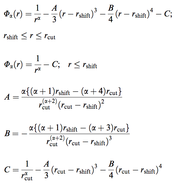
Here α denotes the power of the respective LJ (α=6,12) or Coulombic (α=1) terms. Both potential and force are continuous and smoothly decay to zero between rshift and the cut-off distance rcut. The Martini force field has been parameterized with rshift=0.9 (LJ) or 0.0 (Coulomb) and rcut=1.2 nm.
-
Can I use PME or reaction field with Martini?
In principle you can, although the Martini force field has been parameterized with short range shifted electrostatic interactions. The use of reaction field (which is effectively also a shifted potential) is not likely to affect the behavior very much. PME, on the other hand, may lead to significantly different behavior, and could be more realistic in certain applications (e.g. realistic membrane pores were seen in simulations of both dendrimers [1] and anti-microbial peptides [2] attacking lipid bilayers). Please realize that electrostatic interactions in the Martini model are not considered to be very accurate to begin with, especially as the screening in the system is set to be uniform across the system with a screening constant of 15. When using PME, please make sure your system properties are still reasonable.
However, in combination with the polarizable Martini water model [3], PME can be used and makes sense as the elctrostatic interactions are more realistic.
[1] H. Lee and R. G. Larson, J. Phys. Chem. B, 2008, 112, 7778–7784
[2] A.J. Rzepiela, D. Sengupta, N. Goga, S.J. Marrink, Faraday Discuss., 2010, 144, 431-443.
[3] S.O. Yesylevskyy, L.V. Schäfer, D. Sengupta, S.J. Marrink, PLoS Comp. Biol, 6:e1000810, 2010. open access
-
Can I do free energy calculations with Martini?
Yes you can!
Topologies
-
How do I create a topology for a new molecule?
Here we present a simple three-step recipe, or guide, how to proceed in parameterizing new molecules using the CG Martini model:The first step consists of mapping the chemical structure to the CG representation, the second step is the selection of appropriate bonded terms, and the third step is the optimization of the model by comparing to AA level simulations and/or experimental data.
Step I, mapping onto CG representation: The first step consists of dividing the molecule into small chemical building blocks, ideally of four heavy atoms each. The mapping of CG particle types to chemical building blocks, which are presented in Table III of ref [1], subsequently serves as a guide towards the assignment of CG particle types. Because most molecules cannot be entirely mapped onto groups of four heavy atoms, some groups will represent a smaller or larger number of atoms. In fact, there is no reason to map on to an integer number of atoms, e.g. a pentadecane mapped onto four C1 particles implies that each CG bead represents 3¾ methyl(ene) groups. In case of more substantial deviations from the standard mapping scheme, small adjustments can be made to the standard assignment. For instance, a group of three methyl(ene)s is more accurately modeled by a C2 particle (propane) than the standard C1 particle for saturated alkanes. The same effect is illustrated by the alcohols: whereas the standard alcohol group is modeled by a P1 particle (propanol), a group representing one less carbon is more polar (P2, ethanol) whereas adding a carbon has the opposite effect (Nda, butanol). Similar strategies can be used for modulation of other building blocks. To model compounds containing rings, a more fine grained mapping procedure can be used. In those cases, the special class of S-particles is appropriate.
Step II, selecting bonded interactions: For most molecules the use of a standard bond length (0.47 nm) and force constant of K = 1250 kJ mol-1 nm-2 appears to work well. In cases where the underlying chemical structure is better represented by using different values, there is no restriction in adjusting these values. Especially for ring structures much smaller bond lengths are required. For rigid rings, the harmonic bond and angle potentials are replaced by constraints, as was done for benzene and cholesterol. For linear chain-like molecules, a standard force constant of K =25 kJ mol-1 with an equilibrium bond angle φ = 1800 best mimics distributions obtained from fine grained simulations. The angle may be set to smaller values to model unsaturated cis bonds (for a single cis-unsaturated bond K = 45 kJ mol-1 and φa = 1200), or to mimic the underlying equilibrium structure more closely in general. In order to keep ring structures planar, improper dihedral angles should be added. For more complex molecules (e.g. cholesterol) multiple ways exist for defining the bonded interactions. Not all of the possible ways are likely to be stable with the preferred time step of 30-40 fs (actual simulation time). Some trial-and-error testing is required to select the optimal set.
Step III, optimization: The coarse graining procedure does not have to lead to a unique assignment of particle types and bonded interactions. A powerful way to improve the model is by comparison to AA level simulations, analogous to the use of quantum calculations to improve atomistic models. Structural comparison is especially useful for optimization of the bonded interactions. For instance, the angle distribution function for a CG triplet can be directly compared to the distribution function obtained from the AA simulation, using the mapping procedure described earlier. The optimal value for the equilibrium angle and force constant can thus be extracted. Comparison of thermodynamic behavior is a crucial test for the assignment of particle types. Both AA level simulations (e.g. preferred position of a probe inside a membrane) and experimental data (e.g. the partitioning free energy of the molecule between different phases) are useful for a good assessment of the quality of the model. The balance of forces determining the partitioning behavior can be very subtle. A slightly alternative assignment of particle types may significantly improve the model. Once more, it is important to stress that Table III of ref [1] serves as a guide only; ultimately the comparison to AA simulations and experimental data should be the deciding factor in choosing parameters. Note that you can compare your CG simulations to AA simulations very easily using the Reverse Transformation Tool explained on the tutorial pages.
[1] S.J. Marrink, H.J. Risselada, S. Yefimov, D.P. Tieleman, A.H. de Vries. The MARTINI forcefield: coarse grained model for biomolecular simulations. JPC-B, 111:7812-7824, 2007.
-
How to set-up a protein simulation?
Keeping in line with the overall MARTINI philosophy, the coarse-grained protein model groups ∼4 heavy atoms together in one CG bead. Each residue has one backbone bead and zero or more side-chain beads depending on the amino acid type. The secondary structure of the protein influences both the selected bead types and bond/angle/dihedral parameters of each residue as explained in Monticelli et al. (J Comput Chem Theory, 2008). It is noteworthy that, even though the protein is free to change its tertiary arrangement, local secondary structure is pre-defined and thus static throughout a simulation. Conformational changes that involve changes in the secondary structure are therefore beyond the scope of Martini CG proteins.
Setting up a CG protein simulation consists basically of two steps: 1) converting an atomistic protein structure into a CG model and 2) generating a suitable Martini topology. Both these steps are easy to do with the martinize.py script
-
How do I model DNA and other nucleotides?
We are planning to develop an extension of Martini toward nucleotides, however, this might take a while. For the moment you may have a look at: Khalid S, Bond PJ, Holyoake J, Hawtin RW, Sansom MSP. DNA and lipid bilayers: self-assembly and insertion. J. Royal Soc. Int. 5, S241-S250, 2008.
-
How do I use the polarizable water model and when should I use it?
How? Easy, use the special martini_v2.P.itp file in which the polarizable water model is defined - it also contains the full interaction matrix with all other particles. You can combine it with any other topology file, either 2.0 or 2.1. Only in the latter case please note that particle types AC1 and AC2, used for certain apolar amino acids, are obsolete and should be replaced by norma C1 and C2 particle types. Furthermore, don't forget to set the relative dielectric screening to eps=2.5 instead of eps=15 in standard Martini. See the example mdp file, and also have a look at the example applications featuring a box of pure polarizable water. And last, please have a look at the paper describing the polarizable model:
S.O. Yesylevskyy, L.V. Schafer, D. Sengupta, S.J. Marrink. Polarizable water model for the coarse-grained Martini force field. PLoS Comp. Biol, in press, 2010.
When? We first note that the polarizable MARTINI water model is not meant to replace the standard MARTINI water model, but should be viewed as an alternative with improved properties in some, but similar behaviour at reduced efficiency in other applications. It is 2 to 3 times more expensive than standard Martini because the polarizable water bead has three particles. In combination with PME, which you can do with the polairzable model, it is even slower. However, for systems or processes in which charges or polar particles are present in a low-dielectric medium (e.g., inside a bilayer, or protein), the polarizable water model is much more realistic as it captures the dielectric inhomogeneity of the system. Furthermore, the effect of electrostatic fields (both external and internal) is modeled more realistically. In fact you may even simulate cool phenomena like electroporation.
Problems
-
My simulation keeps crashing, what can I do?
The following is a list of suggestions that might help you stabilize your system:
 Reduce the time step somewhat, some applications require 20 fs rather than 30-40 fs. If you need to go below 20 fs something else is likely to be wrong.
 Increase the neighbourlist update frequency and/or neighborlist cutoff size.
 Replace contraints by (stiff) bonds, recommended during minimization
 Replace stiff bonds by constraints, this will increase stability and allow larger time steps. Stiff bonds are bonds with a force constant exceeding ~ 10000 kJ mol-1 nm-2.
 For beta-strands, you might try using distance constraints, available as option in the itp-generating script. If proteins keep crashing in general, try adding an elastic network to your protein, using ELNEDYN.
 Play with your topology, you might have conflicting bonded potentials. Also make sure you have the appropriate exclusions (nearest neighbours should alway be excluded, but sometimes 2nd or 3rd nearest neighbours as well.
-
My water is freezing, help!
The unwanted freezing of water is a known problem in the current parameterization (version 2). It has already been observed and discussed in our previous work [1,2,3]. Please note the following points:
i) although the LJ parameters for water (ε=5.0 kJ mol-1, σ=0.47 nm) bring it into the solid state region of the LJ phase diagram, the use of a shift potential reduces the long-range attractive part. Consequently, the CG water is more fluid compared to the standard LJ particle.
ii) We have previously [2] determined the freezing temperature of the CG water as 290 +/- 5K. While this is admittedly higher than it should be, in most applications freezing is not observed as long as no nucleation site is formed. Apart from simulations performed at lower temperatures, rapid freezing is therefore a potential problem in systems where a nucleation site is already present (a solid surface, but also an ordered bilayer surface may act as one) or when periodicity enhances the long range ordering (e.g., for small volumes of water).
iii) In those cases in which the freezing poses a problem, a simple pragmatic solution has been presented in the form of antifreeze particles. This works in some cases, but has apparently given problems in combination with solid supports. Therefore, be careful to check that your antifreeze particles do not cluster. You may also switch to the polarizable water model which has a lower melting temperature [4].
Anyhow, the freezing of Martini water is clearly not ideal, and there is room for improvement. In future versions of the MARTINI force field we intend to use a softer potential with a tuneable width to extend the fluid range of the water model.
[1] S.J. Marrink, H.J. Risselada, S. Yefimov, D.P. Tieleman and A.H. de Vries. The MARTINI force field: Coarse grained model for biomolecular simulations. J. Phys. Chem. B, 2007, 111, 7812-7824.
[2] S.J. Marrink, A.H. de Vries and A.E. Mark, Coarse grained model for semiquantitative lipid simulations, J. Phys. Chem. B, 2004, 108, 750–760.
[3] S.J. Marrink, X. Periole, D.P. Tieleman, A.H. de Vries. Comment on using a too large integration time step in molecular dynamics simulations of coarse-grained molecular models. Phys. Chem. Chem. Phys., 12:2254-2256, 2010. abstract
[4] S.O. Yesylevskyy, L.V. Schäfer, D. Sengupta, S.J. Marrink. Polarizable water model for the coarse-grained Martini force field. PLoS Comp. Biol, 6:e1000810, 2010. open access
-
My protein starts deforming, help!
Time to use an elastic network in combination with your Martini protein. See the ELNEDYN tutorial page.
-
My vesicles do not want to fuse, help!
Well, some vesicles simple do not like to fuse so maybe your expectations should be lowered ..... however, there could be a potential artificial barrier toward fusion if you use Martini 2.0 or higher. In order to make the solvation free energy of ions in apolar media more realistic, in version 2.0 the interaction between Q type particles and C1/C2 particles was changed to the 'super-repulsive' category. Here the effective size of the Q particles (or C particles, depending on your perspective) was increased to 0.6 nm, much larger than the standard interaction size of 0.47 nm. This effectively blocked ions from dissolving into apolar solvents such as the bilayer interior. However, it also has the unwanted effect that it hinders lipid tails from protruding toward and through the lipid/water interface. The first barrier to vesicle fusion is the formation of a stalk, which is triggered by the protrusion of lipid tails ...
In order to remove this artefact, simply change the Q-C1/C2 interactions back to their normal 'repulsive' interaction style, but do realize that this will also affect the ability of ions to pass through membranes. If you want to look at fusion in the presence of ions, you might want to add a different particle type to distinguish the Q site of the lipid headgroup versus the Q sites of the ions ..
See also: "Splaying of Aliphatic Tails Plays a Central Role in Barrier Crossing During Liposome Fusion"
D. Mirjanian, A.N. Dickey, J.H. Hoh, T.B. Woolf, M.J. Stevens. J. Phys. Chem. B 2010, 114, 11061–11068, in which this trick was applied.
-
I cannot log-in or post on the forum!
To be able to post on the Martini forum, you have to log-in: From the "User Platform" menu, choose the "Login to Forum". To be able to log-in here, you have to be a registered user. Click the "Register" link at the bottom of the page and provide the required personal data. An e-mail containing an activation link will be sent to the address provided. Check your spam folder in case you did not receive an email!
-
Who can I contact with further questions?
In case you do not find your answer anywhere (FAQ, user platform, tutorial session ...), or if you experience unreported problems, please send an email to:
This email address is being protected from spambots. You need JavaScript enabled to view it.