Physisorption on particle-based surfaces
- Details
-
Last Updated: Thursday, 21 November 2019 15:04
Self-assembly of functionalized alkanes on a graphite surface
This tutorial guides you on how to perform self-assembly simulations on a graphite flake using a special version of the coarse-grained force-field MARTINI [1], similar to work done in publication [2]. The Martini force-field was originally developed for lipids [1] and then extended to many other systems including self-assembly on a graphite flake [2,3]. For learning purposes, we will limit ourselves to a tiny graphite flake with a small number of adsorbent molecules. Such simulations can be done on a personal computer within 2h. The tutorial is prepared for GROMACS 2016 versions and may need (small) changes in other versions. All files for this tutorial can be found in this zip file.
The aim of the tutorial is two-fold:
- it contains specific information to set up the self-assembly simulations of long-chain functionalized molecules on graphite
- it contains a method to construct a regularly packed surface consisting of a number of layers of beads: this method can be used to construct any such surface or crystal regardless of the nature of the beads or application
This tutorial assumes a basic knowledge of the Linux operating system and some experience with gromacs. It is helpful to have a basic understanding of the gromacs molecular dynamics package and the Martini force-field. You can find tutorials on these topics at http://cgmartini.nl and http://www.mdtutorials.com/gmx/lysozyme/index.html.
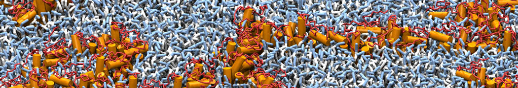
In this tutorial, we will perform a simple simulation of self-assembly (that is adsorption and rearrangement) on a graphite surface from a random configuration of adsorbent in a solvent. We will study here self-assembly of a linear functionalized alkane, AM25, which consist of 6 beads (two P1 polar and four C1 apolar beads, respectively, arranged as C1-P1-C1-C1-P1-C1), which can represent N,N′-decanomethylenebispentamide (C4H9-CO-NH-(CH2)10-NH-CO-C4H9). For more information, look into publication [2]. As a solvent, we use phenyloctane, which in its coarse-grained representation consist of 5 beads (three SC4 beads in a ring and two C1 beads in a tail)
0. Setting up the system
Download the zip file, and unzip it. It expands to a directory or folder called Tutorial. Go into the folder of the tutorial. For purposes of this tutorial this will be our working directory:
$ cd Tutorial
Make an empty directory in which you will test the simulation protocol:
$ mkdir testSA
$ cd testSA
First copy a sample topology file:
$ cp ../topology/sample_topol.top topol.top
The topology file consist of references to parameters of force-fields and number of molecules in the system. Here is the sample_topol.top file:
#include "../FF/martini_v2.15.itp"
#include "../FF/martini_v2.0_solvents.itp"
#include "../FF/martini_v2.0_graphite.itp"
#include "../FF/martini_v2.0_graphite.itp""
[ system ]
Adsorption on graphite
[ molecules ]
GRAP 1600
AM25 50
PHEO 300
The first four lines describe where parameters of force-field can be found (in subdirectory "Tutorial/FF"), then there is [ system ] with a title of simulation, and then [ molecules ], after which there are types and numbers of molecules of each type used in the simulation. For this tutorial, we use 1600 beads of graphite, 50 molecules of AM25, and 300 molecules of solvent PHEO. The subfolder "Tutorial/topology" also contains other topologies used in publication [2].
Copy the coordinate file of a small graphite flake from the "Tutorial/gro" folder (to learn how to make a graphite flake yourself look at the end of this tutorial page). This box contains 1600 graphite beads in four layers, arranged in a hexagonal pattern. The beads are located inside the box, making sure there is space between the periodic images in all directions. This is why it is called a "flake", as opposed to a "surface". In many modeling applications, surfaces (of solids) are modeled as periodic entities, with a number of unit cells explicitly described and connected across the periodic boundaries. Here, this is NOT the case.
$ cp ../gro/small_graphite.gro 0_box.gro
Insert adsorbent molecules into this box using the "gmx insert-molecules" command: the coordinate file for single molecules of adsorbents are in the "Tutorial/gro" subdirectory. Here, we insert 50 adsorbent molecules of the AM25 kind:
$ gmx insert-molecules -f 0_box.gro -ci ../gro/AM25.gro -o 0_box_ad.gro -nmol 50
Add solvent molecules using the "gmx solvate" command: here we use the -maxsol option to limit the number of molecules to 300 (however, you don't have to use it, but you have to then make an appropriate change of the number of molecules in topol.top file):
$ gmx solvate -cp 0_box_ad.gro -cs ../gro/phenyloctane.gro -o 0_box_sol.gro -p topol.top -maxsol 300
The subfolder "pictures" includes snapshots of different stages of the processes filling the box.
Now it is time to perform simulations with the system prepared.
1. Energy minimization
After our system is set up, perform energy minimization, to remove all bad contacts (which could result in numerical instability and an explosion of the system). All parameter files for the simulation engine are in the "Tutorial/mdp" folder. All *.mdp files are similar to one present on other tutorials of Martini except lines in which we specify that graphite beads are frozen (freezegrps = GRAP and freezedim= Y Y Y). The graphite beads do not move during the course of simulation (but they do interact with adsorbent and solvent molecules). This is a choice that is usually made to limit the computational effort. The graphite surface when run without the "freezegrps" option is stable at small time-steps, but defects might occur over time.
$ gmx grompp -f ../mdp/1_em.mdp -c 0_box_sol.gro -p topol.top -o 1_em.tpr
[
Note that you may have to ignore WARNINGS. This can be done by adding the -maxwarn option to the gmx grompp command, e.g. if you need to ignore 1 warning:
$ gmx grompp -f ../mdp/1_em.mdp -c 0_box_sol.gro -p topol.top -o 1_em.tpr -maxwarn 1
]
$ gmx mdrun -v -deffnm 1_em
[
Note that here you may have to limit the number of threads because the system is quite small, and may be too small for the domain decomposition over the available number of nodes. To use 4 threads, for example:
$ gmx mdrun -v -deffnm 1_em -nt 4
]
Energy minimization will produce an local energy minimized structure in the 1_em.gro file, which we use for further simulations.
2.Equilibration
We perform the equilibration in two stages: first we equilibrate at constant volume and temperature (NVT ensemble) and then at constant pressure and temperature (NPT ensemble).
Equilibrate the system in the NVT ensemble:
$ gmx grompp -f ../mdp/2_nvt.mdp -c 1_em.gro -p topol.top -o 2_nvt.tpr -maxwarn 1
$ gmx mdrun -v -deffnm 2_nvt
We use the option "-maxwarn 1" to ignore one warning:
WARNING 1 [file ../mdp/2_nvt.mdp]:
For proper integration of the Berendsen thermostat, tau-t (0.3) should be at least 5 times larger than nsttcouple*dt (0.3)
which we ignore because we are performing this step to get a reasonable starting structure for production simulations and are not too concerned that the statistical ensemble or integration is not exact.
Equilibrate system in the NPT ensemble:
$ gmx grompp -f mdp/2_npt.mdp -c 2_nvt.gro -p topol.top -o 2_npt.tpr -maxwarn 2
$ gmx mdrun -v -deffnm 2_npt
In this case, we use "-maxwarn 2" to ignore two warnings:
WARNING 1 [file ../mdp/2_npt.mdp, line 65]:
All off-diagonal reference pressures are non-zero. Are you sure you want to apply threefold shear stress?
We ignore it because we want to allow deformations of the box only in the z-direction (the direction perpendicular to the plane of the graphite flake. The flake should not come near its periodic image, and therefore the lateral (x, y) directions are kept fixed.
WARNING 2 [file ../mdp/2_npt.mdp]:
For proper integration of the Berendsen thermostat, tau-t (0.3) should be at least 5 times larger than nsttcouple*dt (0.3)
3. Run simulation
After the temperature and pressure of the system are equilibrated, it is a time to perform a production simulation:
$ gmx grompp -f ../mdp/3_run.mdp -c 2_npt.gro -p topol.top -o 3_run.tpr -maxwarn 2
$ gmx mdrun -v -deffnm 3_run
This command will produce several files, from which final structure is in 3_run.gro and trajectory in 3_run.xtc file. Such a simulation on a PC (CPU Intel(R) Core(TM) i7-5600U CPU @ 2.60GHz) takes about 2h.
You can visualize this trajectory and structure using visualization program such as VMD (http://www.ks.uiuc.edu/Research/vmd/). A quick impression of the system can be gotten with "gmx view" if you have installed it (not standard!):
$ gmx view -s 3_run.tpr -f 3_run.xtc
Select which molecules you want to see, and find the "Display/Animate" tab to click through the trajectory. If you are happy, you can spend more time on better visualization, for example using VMD. It is recommended that you first convert your trajectory, (1) to avoid long bonds appearing between beads that are on the other side of the periodic box ("-pbc whole"), and (2) to make VMD draw bonds between beads that have much longer bond-lengths than the standard cut-off of VMD ("-o 3_run.tng"; the .tng format knows which bonds to draw and makes the plug-in "cg_bonds.tcl" largely obsolete).
$ gmx trjconv -f 3_run.xtc -pbc whole -o 3_run.tng
$ vmd 3_run.tng
This concludes the tutorial on the set-up of a small system for 2D self-assembly on graphite from solution. In this tutorial, you were given a small graphite flake in a simulation box. Here is how you can make your own!
4. Custom size of graphite flake:
NOTE that the following procedure can be used to create any regular arrangement of beads given a unit cell!
In the main directory Tutorial, make a new folder for testing:
$ mkdir testFlakeSetup
$ cd testFlakeSetup
You can make a custom size of the graphite flake from the unit cell given in the "Tutorial/gro" subfolder file "cell.gro"; this cell contains just two beads from which a graphite flake can be produced using the command:
$ gmx genconf -f ../gro/cell.gro -nbox 20 20 2 -o 0_out.gro
This creates rhombic graphite flake of 20x20 unit cells in the x- and y-directions and two unit cells (four layers) in the z direction (the cell contains two beads in the z-direction). Subfolder "Tutorial/gro" also contains a coordinate file (graphite_paper.gro) of the graphite flake used in publication [2].
Next, create a simulation box with a given size:
$ gmx editconf -f 0_out.gro -o 0_box.gro -box 7 7 7 -angles 90 90 60
The "-angles" option causes the simulation box to be hexagonally shaped in the x-y dimension (as is the flake), and with right angles to the z-direction. It is essential that the simulation box is larger than the graphite flake (the periodically connected graphite surface causes packing artefacts).
Having created your own box, you can use it to fill with adsorbents and solvent, or do other cool things you might think of...
5. Simulation of other molecules:
Since some of the parameters for simulation engine reference to a specific group of molecules, to simulate different molecules, you need to make appropriate changes in mdp files. For example, if you would like to simulate AL1 molecules, you can do it using one simple command. You may want to keep the existing mdp files, so...
In the main directory Tutorial, make a new folder for testing:
$ cp -R mdp mdp-AL1
$ sed -i 's/AM25/AL1/g' mdp-AL1/*mdp
which changes all the names of molecules AM25 to AL1 in mdp files.
The coordinate files for the different adsorbents are in "Tutorial/gro" subfolder.
References:
[1] Marrink, S. J., Risselada, H. J., Yefimov, S., Tieleman, D. P., and De Vries, A. H. (2007) The MARTINI force field: coarse grained model for biomolecular simulations. J. Phys. Chem. B 111, 7812–7824.
[2] Piskorz, T. K., Gobbo, C., Marrink, S.-J., Feyter, S. de, Vries, A. H. de, Esch, J. H. van (2019). Nucleation mechanisms of self-assembled physisorbed monolayers on graphite. J. Phys. Chem. C, 123, 17510-17520.
[3] Gobbo, C., Beurroies, I., De Ridder, D., Eelkema, R., Marrink, S. J., De Feyter, S., De Vries, A. H. (2013). MARTINI model for physisorption of organic molecules on graphite. Journal of Physical Chemistry C, 117(30), 15623-15631.
Tutorial contributed by Tomasz K. Piskorz.
Martini tutorials: polymers
- Details
-
Last Updated: Monday, 24 August 2015 14:05
Martini tutorials: polymers
Summary
General aspects
Parametrization of a polymer melt: 200 PEG 9mers at 300K
Mapping
Coarse-graining the atomistic trajectory
Extraction of properties and bonded distributions (atomistic)
Creation of an .itp file
Energy minimization and simulation of the system
Extraction of properties and bonded distributions (CG)
Back to the drawing table
What next
Free-energy verification
Backmapping
General aspects
Parametrization of polymers follows pretty much the standard procedure for the parametrization of any other molecule. There are, however, some factors to consider:
Sometimes you'll want a polymer to reproduce certain particular features known from experimental observations or atomistic simulations. These features can be, for example, a target radius-of-gyration or helical propensity. These often depend on more bonded and nonbonded interactions than those dealt with when parametrizing simpler molecules. Try including longer-range distances and angles as targets distributions, and understand what may be preventing your CG polymer from following those.
When dealing with an oligomer, the behavior of residues close to the termini is often not representative of that of the rest of the molecule. It is a good idea to obtain reference distributions from a polymer chain long enough that a consistent behavior is obtained for the central residues. If the termini behave very differently, it might be worth assigning a different set of potentials to those.
You may find that Martini cannot faithfully reproduce the long-range structural organization you aim for, no matter how many potentials you use or how finer you make the mapping. Before you throw in the towel it can be an acceptable approach to use an elastic network to restrain the beads to the conformation you want (see the example of proteins). The flexibility afforded by the network is tunable, and might be enough to satisfy your needs.
Some polymers can establish different intramolecular dipole interactions or salt bridges depending on conformation (think carbonyl–amide h-bonding in proteins). A single set of bead types may then be insufficient to describe the effective polarity of all the conformations of the polymer. This requires a different bead type assignment for each conformation, just like the polarity of backbone beads in Martini proteins depends on their secondary structure. Beware that such an assignment is static, and won't change during a simulation if the conformations change. This approach is therefore most useful when you are sure that the polymer conformation will be kept (for instance, when restraining it with an elastic network).
In the case of polymer melts — or even when using small molecules as a solvent — achieving the right density becomes important. The iterative parametrization steps should take this into account.
When parametrizing polymers of varying length and residue composition, matching of partition behavior is probably best done on a per-residue/fragment basis, rather than whole molecules. This should give the most transferrable behavior.
Parametrization of a polymer melt: 200 PEG 9mers at 300K
In this tutorial we carry out the Martini parametrization of a PEG9 molecule from target atomistic data. The focus will be to match the mapped distribution of bonded conformations, as well as average density and molecular radius-of-gyration. For the time being, bead assignment will be only done to match the Martini building blocks — without adjustment for the matching of partition properties.
This exercise will involve the use of several GROMACS tools as well as some scripting (example scripts are provided, but beware that they were made specifically for this tutorial and will most likely not work for parametrizing other molecules without modifications). We will deal with some of the issues faced when parametrizing new molecules in general, and some particular to polymers. It is very useful to quickly read through the tutorial on molecule parametrization (particularly the flowchart in that page), as it sets out most of the general Martini parametrization workflow. Finally, in this tutorial we suggest some filenames, but these are by no means binding. Each user should feel free to adapt them to their organization scheme.
Martini models of PEG have already been published (see Lee et al. or the newer Rossi et al.) The aim of this tutorial is not to supplant them but rather to provide an example workflow of parametrization. For the same reason an automatically generated topology was deemed sufficient for generating the target atomistic data.
The atomistic target data
We start off with the target atomistic trajectory of the system to parameterize. In the PEG_parametrization.tgz file you'll find the AA directory containing a 100ns trajectory of a melt of 200 PEG 9mers. These data were obtained from a PEG9 topology generated by the Automated Topology Builder for the GROMOS 54a7 united-atom forcefield; you'll find it under PEG9.itp (the naming and atom order were slightly modified compared to the .itp in the ATB repository, but the potentials are unmodified). Be sure to take a look at the .itp file to have an idea about the atom ordering and naming in the molecule.
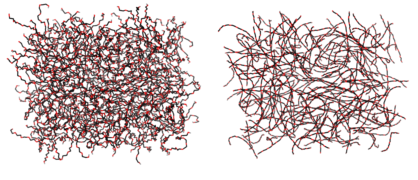
Figure 1 | Different visualizations of the AA polymer melt. Left: single snapshot after almost 100ns of simulation. Right: Time averaged (200 ps) ensemble around the same time point as for the left panel.
Mapping
With the atomistic data at hand it is time to decide on an AA-to-CG mapping. Each ethylene glycol residue consists of two methylenes and an ether oxygen (in our target data, which comes from an united-atom topology, the methylenes are represented by a single particle each). A reasonable mapping strategy is then to assign each residue to a CG bead. This results in a 3-to-1 mapping, slightly finer than the typical 4-to-1 of Martini. Alternatively, two residues can be assigned to a single bead, for a 6-to-1 mapping. Figure 2 depicts different possible mapping strategies for PEG. Note that in the first mapping, where each bead corresponds to an O-C-C sequence, the terminal assignments become asymmetric. This is undesirable given the symmetric nature of the polymer.
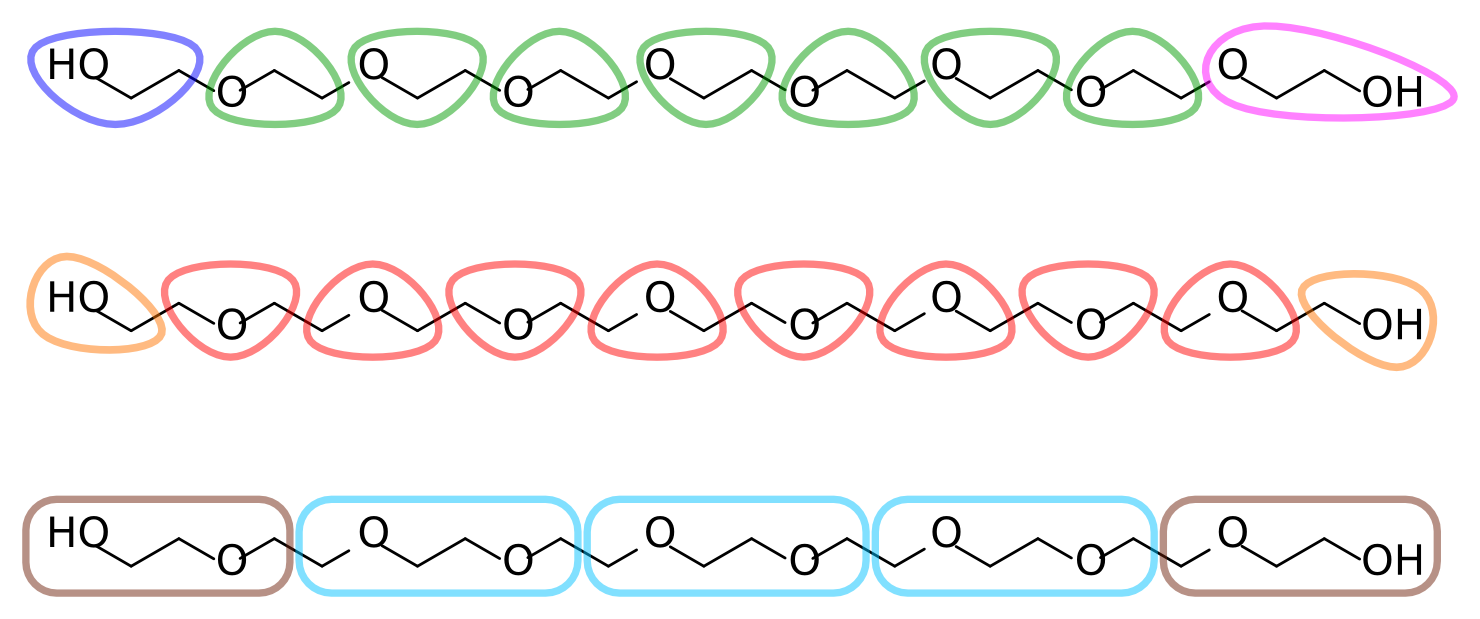
Figure 2 | Different mapping strategies for PEG9.
The remainder of this tutorial uses the second mapping strategy from Figure 2, where each bead corresponds to a C-O-C sequence, with two smaller but symmetric C-O-H assignments at the termini. Feel free to follow your chemical intuition and choose a different mapping; this will make it more challenging and potentially interesting, as you'll have to adapt more of the tools and files that are provided.
Coarse-graining the atomistic trajectory
Using the chosen mapping we can proceed to transform sets of atomistic coordinates into CG ones simply by finding the center of mass of each group of atoms in a CG bead. There are different ways to proceed with this so-called "forward mapping".
The first method uses the GROMACS tool g_traj to output centers of mass of arbitrary selections as a function of time in trajectory format. This requires that an index file be created containing one group per bead, each group listing the respective atomistic atoms. As you can imagine for a system such as ours this index file requires a bit of scripting to prepare as there'll be 2000 groups (or as many CG beads as your mapping yields). The script indexer.py will do this for you, but edit it to understand its workings and to ensure its parameters are correct for the mapping you chose. To use g_traj, ask for 2000 groups, set the -com flag, and point it to the PBC-treated AA trajectory, the compiled topology, and the index we just prepared:
seq 0 1999 | g_traj -f AA/trajpbc.xtc -s AA/topol.tpr -oxt traj_cg.xtc -n mapping.ndx -com -ng 2000 -b 20000
g_traj will prompt you for which index groups correspond to the 2000 that were asked with the -ng flag. By piping the output of seq 0 1999 into it we automate the process and ensure they are output in the correct sequence. Here we also used the -b flag to discard the first 20ns as equilibration time. g_traj yields an .xtc trajectory file. To serve as a starting point for CG simulations later, and also for visualization and analysis purposes, it is useful to also have a .gro file; the same g_traj command can be adapted to that end, by setting -b 100000 to only pick the last frame and choosing an output filename with the appropriate extension:
seq 0 1999 | g_traj -f AA/trajpbc.xtc -s AA/topol.tpr -oxt cg.gro -n mapping.ndx -com -ng 2000 -b 100000
The second forward mapping method, which we won't cover in detail here, makes use of the backward tool. This script was developed to automate the backmapping of CG structures to atomistic, but can also perform forward mapping. It uses mapping files to decide which atoms to calculate centers of mass from, and is therefore more flexible than the approach above. It is of particular interest when dealing with polymers with arbitrary sequences of different residues, for which the scripting of the indexation is not as straightforward.
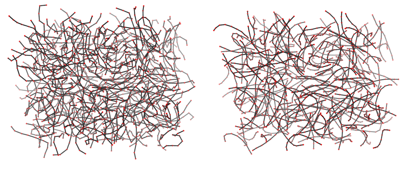
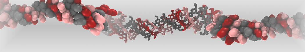
Figure 3 | Different visualizations of the center-of-mass-mapped AA polymer melt. Red spheres are the centers of mass; bonds are dark grey. Same panel setup as in Figure 1.
Extraction of properties and bonded distributions (atomistic)
Armed with mapped .xtc and .gro files you can now use g_bond and g_angle to extract the relevant bonded distributions of the beads. To this end index files will have to be generated specifying which bonds/angles/dihedrals to measure (see the -h flag of each command). Again, the generation of thousands of atom pairs (for bonds), triplets (for angles), or quadruplets (for dihedrals) requires some scripting, and the gen_indices.py script is there for you. If you inspect the code you'll notice that the indices will be split between _core and _term groups. These groups separate bonded interactions involving the termini from those that only contain core beads. This might be desirable because a) the termini were mapped differently than the rest of the molecule, and b) even if they were mapped just as the core beads, termini often explore different or more extreme bonded configurations.
Now invoke each analysis tools on each index group; remember to change the output filename when selecting the termini and the core groups, in order not to clobber results:
g_bond -f traj_cg.xtc -blen 0.35 -tol 0.8 -n bonds.ndx -o bonds.xvg
g_angle -n angles.ndx -f traj_cg.xtc -od angdist.xvg
g_angle -type dihedral -n dihedrals.ndx -f traj_cg.xtc -od dihdist.xvg
You'll be repeatedly running these same commands later when attempting to reproduce these distributions. The bash script calc_dists.sh does that for you; just be sure to adapt file names and locations.
Now view the distributions you obtained. Compare the termini with the core ones and decide which will warrant different potentials and which can be treated as the same. You can also at this point predict the distributions that can be problematic to reproduce:
those that are obviously multimodal, with spread apart modes;
those that are concentrated around a very narrow parameter space and will therefore require very strong potentials;
and the dihedrals that span bond angles that can extend to 180 degrees.
At this point it is also a good idea to calculate the density of the atomistic system, as we'll be wanting to match it as well (you can instead try to match the known experimental density, if you have it). If an .edr file is available one can use the g_energy tool to this end. However, in the absence of an .edr file one can simply use
g_traj -f traj_cg.xtc -ob box.xvg -s cg.gro
which will extract the box vectors as a function of time. These can then be averaged using g_analyze:
g_analyze -f box.xvg
The average volume can be calculated from the first three averages (which correspond to the average X, Y, and Z box sizes, respectively, in nm). From the average volume you can readily calculate the average system density.
As an additional parametrization target we'll be aiming to reproduce the radius of gyration of the atomistic PEG molecule. You can use the g_polystat tool to calculate it, but it requires a .tpr file to know the number of atoms per molecule. The best is to leave this for now and calculate it later when you get a .tpr for the CG runs, which will have appropriate molecule information.
Creation of an .itp file
For this step it might be useful to use the .itp of a preexisting molecule as a template for your own (take your pick from the several available at the Martini website). Since there will be an iterative optimization procedure involving several attempts at this file, it is wise to start off by placing it in a subdirectory (take0 seems an appropriate name). This will keep chaos from ensuing when generating new trajectory and distribution files, which would get mixed with the atomistic ones or with those from other iterations. This tutorial assumes you'll be working in a subdirectory for each take.
[ moleculetype ]
Under the [ moleculetype ] directive you should input the name for your molecule. This is the name you'll be referencing in the .top file. Next to the name is the default number of bonded neighbors that are excluded from nonbonded interactions. Standard Martini procedure is to exclude only first bonded neighbors, by setting this value to 1. Should more exclusions be required it is usually best to add them individually later in the topology.
[ atoms ]
This directive defines the atom properties of the molecule. Remember that in our CG system molecules have 10 atoms (beads). At this point atom and residue naming are of little importance (but remember, 5 character limit). The atom types, however, control the nonbonded interactions and are a central part of the coarse-graining process. Again, you'll use your chemical intuition, and a copy of the 2007 Martini paper, to judge which bead type better represents each mapped moiety: find Table 3 in the paper, and in there find the building block that most closely matches the one underlying each bead. For the C-O-C mapping it is probably one of the N* bead types, whereas for the termini one of the P* ones. A correct choice means that the interaction of a bead with different solvents follows the correct partitioning energies (see the solvents used for parameterization in the paper's Table). The idea behind Martini is that, by matching this partition behavior, we will get a consistent strength of nonbonded interaction between the bead types in the Table.
Martini also provides the so-called S-beads (SP*, SN*, etc.). These are smaller versions of regular beads that can pack closer together but with a shallower nonbonded energy well that keeps them from solidifying. They are typically used for mappings finer than 1-to-4, and might be useful in our case if the density of the system turns out to be too low. Be aware that these beads only pack closer to other S-beads. Interaction with regular beads follows the same potential as between regular beads.
For the rest of the [ atoms ] directive be sure to set all beads to 0.0 charge and to assign each to their own charge group. Leave masses blank for the default value. When coarse graining, our bonded parameters aim to reproduce statistical averages and not the frequency of real quadratic or cosine oscillations; the meaning and importance of bead mass is therefore less strict as for atomistic forcefields.
[ bonds ], [ angles ], [ dihedrals ]
Now the begins the trial-and-error part of the procedure. Write down for each relevant section the atoms involved in the potential, the function number, and your first guess for the equilibrium value and potential force.
Martini typically uses type 1 bonds, and forces usually fall in the 103 kJ/mol‧nm2 range.
Angles are typically type 2, as these don't get unstable at 180°. Forces usually fall in the 102 kJ/mol range.
Finally, dihedrals are typically assigned either type 1 (with forces in the 100 kJ/mol range) or type 2, when keeping structures like rings planar (forces in the 102 kJ/mol‧rad2 range).
This said, you, as supreme parametrizer of your system, have full choice over which potentials to use (even non-analytical tabulated ones are possible, although they are a bit off the scope of this tutorial). However...
*** DIFFICULTY WARNING ***
This mapping involves bond angles that can reach 180°. Applying dihedral potentials over these bonds will lead to severe instabilities. We recommend, for the sake of finishing the tutorial in a timely and successful fashion, to skip the reproduction of the dihedral distributions. If you dare go down that path take the following advice:
Use stronger angle potentials that prevent beads from becoming colinear (the type 1 angle might be an option here);
Use a smaller simulation timestep than the typical 20fs, to give those angle potentials a chance to act on the molecules;
Try out the new restricted bending angle potentials that we just implemented in version 5.0 of GROMACS! They avoid colinear bonds without requiring any lowering of the timestep or changes to the dihedral potentials.
With that out of the way, we're ready to test-drive our brand-new CG molecule (no more directives should be needed in the .itp file).
Create a .top file that #includes the martini_v2.2.itp file (this is where bead interactions are defined) as well as the PEG .itp you just created (you can use the atomistic topol.top as a template). Specify how many molecules you have in the system, and you're done.
Energy minimization and simulation of the system
The first step is to generate a CG configuration stable enough to start a simulation from. Use the supplied em.mdp together with the just-created .top file and the cg.gro you forward-mapped earlier:
grompp -f ../em.mdp -p topol.top -c cg.gro
You will likely receive a warning that your atom names do not match. This is ok to ignore as long as you understand why that difference arises (and you do, right?). Just rerun the grompp command with the -maxwarn 1 flag, and minimize the structure with:
mdrun -v -rdd 1.4 -c em.gro
After finishing mdrun will dump the minimized coordinates as the em.gro file. Note the use of -rdd 1.4. This tells GROMACS, when parallelizing, to search a bit further into neighboring cells for bonded partners. This might not be required in your case, and there is a performance penalty associated with it. If however it is needed and you leave it out, you'll get spurious error messages complaining about "missing interactions".
At this point it is instructive to read em.mdp and see the options required for Martini. In this particular case the electrostatic treatment is not necessary as we don't have charges in our system. Also note that the typical smoothness of Martini potentials lets us use the straightforward steepest descents minimization (integrator = steep in the .mdp) without fear of letting the system get trapped too far away from the energy minimum.
From this point, prepare the MD run with:
grompp -f ../md.mdp -p topol.top -c em.gro
You should get no further warnings about atom names, since they are sorted out in em.gro. You might, though, be warned that your timestep is too large for the predicted frequencies generated by some of your bonded potentials. If this is your first try, do lower the force constants in question. If you got to these warnings after having to use a high force constant to match bond distributions, it might be a good idea to replace them by constraints. You might also get warnings about the not-so-weak coupling nature of the thermo- and barostats if you decrease their time constants. These are usually safe to ignore with Martini, although it will be up to you to demonstrate that pressure and temperature behavior is adequate.
You can now (finally!) run the MD simulation of your parametrized PEG!
mdrun -v -rdd 1.4
Take the time of your simulation to read the .mdp file and understand its thermostatting and barostatting options. Martini has traditionally been coupled to the berendsen thermo- and barostats, although other scheme combinations can be used. The robustness of Martini and of the berendsen schemes allows one to skip, for most simple cases, any NVT pre-equilibration.
If you get errors at this point there can be multiple causes, and GROMACS is not always able to exit cleanly and in an informative way. The most frequent cases are:
Dihedrals, or type 1 angles, over bonds that become colinear;
Tight networks of constraints that cannot be respected properly for the given timestep or for the requested accuracy in the .mdp (see the lincs_order and lincs_iter options);
Misconstructed or not properly minimized starting configurations.
There can be, of course, many other causes for instability. Reducing the timestep often helps, but this is undesirable (aim for the typical Martini step of 20fs). Sometimes running a short NVT simulation at a low timestep allows the system to become stable enough to continue in NPT at higher timesteps. In addition, a good diagnosis process is to create an .mdp that outputs every simulation step. This will let you identify precisely the events that lead to a crash.
When you get a stable run it is time for...
Extraction of properties and bonded distributions (CG)
At this step you will simply rerun the analysis tools on the CG trajectory. Very importantly, prior to analysis you must make your molecules whole across the PBC:
trjconv -f traj.xtc -pbc mol -o trajpbc.xtc -b 1000
The -b flag discards the first 1 ns as equilibration time. You can now use the calc_dists.sh script but be sure to adapt it for file locations.
Also calculate the system density. Unless you used tailored bead masses, g_energy won't be able to report it correctly. Get the average volume by simply running g_energy on the output ener.edr file, and compute the density using the known system mass.
Finally, use g_polystat to calculate the average radius of gyration of the polymer chains. With the .tpr from this run you can now also calculate the atomistic radius of gyration, if you haven't already done so.
Back to the drawing table
Now use your favorite plotting tool to compare distributions to the target atomistic ones. Also compare the average densities and radius of gyration.
It is unlikely you nailed all the distributions and target properties spot on on the first try. It is then time to create a take1 directory and populate it with the files required for a new run. Copy over the PEG .itp and adjust it based on the distribution/property discrepancies. A good idea, to prevent long equilibration times, is to use the endfile of the previous take as the starting configuration for the new parameterization test run. Just beware of runs that end up in obviously unstable configurations, or that undergo unwanted phase transitions.
An important note when parametrizing solvents or, in this case, melts, is to check the density for too large deviations from the target value. Differences of more than 5-10% are difficult to correct alone by adjusting the bonded potentials, and you'll probably have to rethink the bead types you're using.
Repeat until you are satisfied with the results you've got. When that happens, congratulations, you've parametrized your first Martini polymer! Go drink a Martini to celebrate.
What next?
Free-energy verification
In our approach we focused on reproducing the bonded behavior of the polymer. The nonbonded part was addressed by choosing Martini building blocks that represent the chemical nature of PEG and that yield its correct density. The Martini philosophy, however, calls for a more careful approach where the partition properties of the resulting molecule are checked against experimental or simulated data.
Typically, free-energy is matched to partition data taken between aqueous and apolar solvents. This stems from Martini's origins as a forcefield for biomolecular simulations. It should be stressed, however, that this sort of parametrization must be adapted to the problem under study. If, for instance, the model's application concerns mostly interaction with hydrophobic molecules, then it's the partition into and among those that should be aimed for.
Melt-Water partition
The solvation free energies of our PEG9 molecule have been determined by thermodynamic integration (TI) at the fine-grain level. You can access that data here. The same archive contains a CG directory with H2O and Melt subdirectories ready for you to populate with your systems.
In each directory you will perform simulations to calculate the respective solvation free energy. You will do this by decoupling the nonbonded interactions between solute (a single PEG9 molecule) and each of the solvents. This decoupling will be done gradually, over 10 steps, so that it is possible to calculate a free energy difference between each. You will need the .itp file of the topology you optimized for PEG9, and two .top files: one for the melt system and another one for a 1 PEG + several waters.
System initialization
You can use a .gro file from the end of your parameterization as a starting point to calculate the solvation energy of PEG9 into its own melt. However, we need to tell GROMACS we want to decouple one molecule from all the others.
GROMACS has several ways of specifying a switching between coupled and decoupled states. Here we do it by passing the name of the molecule to decouple to the couple_moltype option in the .mdp. However, in the case of a melt this would mean all molecules would become decoupled simultaneously. The workaround for this is to copy your PEG .itp file to another name, and in there change the molecule name (let's say PEG9X). This will allow you to specify in your .top file the two "different" molecules separately:
[ molecules ]
PEG9X 1
PEG9 199
For the water system you need to create a .gro file with a solvated PEG9 chain. An easy shortcut is to use the same .gro file as for the step above but changing the .top to become:
[ molecules ]
PEG9 1
W 1990
This will tell GROMACS to interpret any atoms after the first PEG as water beads. You will then need to equilibrate this system for a short period before using it for TI (use the provided eq.mdp file).
Simulation setup
To switch between the coupled and decoupled states we define in the .mdp 11 states, each with a different scaling of the Van der Waals interactions (more steps would be required to switch off Coulombic interactions, but there are none in our system). The scaling is defined by variable lambda, varying between 0 and 1. The meaning at lambda=0 and lambda=1 is set with the couple-lambda0 and couple-lambda1 in the .mdp. In our .mdps lambda=0 means a full Van der Waals coupling (couple-lambda0=vdw) while lambda=1 means a fully decoupled molecule (couple-lambda0=none).
The lambda values at each of the 11 different states are given with the vdw-lambdas .mdp directive; the init-lambda-state directive tells GROMACS which of the 10 to actually use in a particular run. The simulations will periodically output the potential energy of the system (the frequency being controlled by the nstdhdl directive). The analysis method we'll be using requires that for a given state the energies of the same configuration under all other states' Hamiltonians also be output. This is set with calc-lambda-neighbors=-1 (and is also why every run needs to know which other states there are).
You'll find a TI.sh script in each of the H2O and Melt subdirectories. This file automates the generation of the 10 systems to be run. Read it carefully to understand how it changes the .mdp file for each decoupling step (hint, look for the sedstate label, that'll be used by the sed command to create the different step files). Also notice how it links the output dhdl.xvg files to the root directory for further analysis.
Integration with MBAR
We'll be using the MBAR integration and error-estimation method (see a detailed description of the method, and the used analysis scripts at the AlchemistryWiki). A python script for analysis is provided, but it requires the pymbar package. If it's not yet installed can do so with
sudo pip install pymbar==2.1.0-beta
(if you don't have sudo privilege in your workstation you can install pymbar locally to your home directory by also passing the --user flag)
After all runs are complete run, inside the H2O and Melt directories, the provided alchemical-gromacs.py script (from http://github.org/choderalab/pymbar-examples), telling it the output filename prefix (-p flag) the temperature (-t flag) and how many ps to leave out as equilibration time (-s flag; 1000 ps was deemed enough):
python ../../alchemical-gromacs.py -p dhdl -t 300 -s 1000
The results will provide calculations using different methods. You should use the ones from MBAR. The script output files will also let you see the individual free-energy changes between steps, and identify areas where more lambda points should be run to lower the estimate error (but beware that because of the need to evaluate energies at all the steps' Hamiltonians if you add more lambda points all steps will have to be rerun).
Backmapping
After the successful parameterization and simulation of your new molecule you may want to convert it back to fine detail (for instance, to proceed with a fine-grain simulation after equilibrating the system with CG). This process is called backmapping.
Due to the reduction of degrees of freedom involved in coarse-graining, the reverse process is not uniquely defined: there will be multiple atomistic configurations that can correspond to a CG grain structure. However, knowledge of the atomistic topology allows us to input more data into the process: an initial atomistic configuration is prepared where atoms are randomly placed in the vicinity of the repective CG bead. The system is then allowed to energy-minimize and equilibrate subject to some restraints. The bonded information contained in the topology leads this process into providing a consistent fine-grain configuration compatible with the starting CG one. Before continuing you can read more about the procedure here and here.
To reverse-map your coarse-grain PEG system you'll need the backward tool, available here. Unpack it into a new folder. Now copy over to the same folder the CG .gro file together with the fine-grain .top and the PEG9.itp referenced in the .top file. This is enough information to recreate a GROMOS 54a7–compatible structure.
We must now teach our PEG mapping to the backmapping procedure. This is done by creating a .map file. The format is described here, but you may start by copying a preexisting file from the Mapping directory (you can also find a ready example in the root of the tutorial directory you downloaded).
In the .map file you'll want to name your [ molecule ] as the name you used for each CG PEG residue. If you named your residues differently (say, to distinguish terminal ones) it is best to edit your CG .gro file and set them all to the same name.
Under the [ martini ] directive you'll enter the name of the bead(s) that compose each residue. In our case each residue is composed by a single bead. Again, these beads should all have the same name in the .gro file; edit it if needed.
The [ mapping ] directive lists which force-fields this mapping is set for. It serves as a tag for when multiple mappings are available, and to let the script know what is the level of detail of the target forcefield (coarse-grained, united-atom, or all-atom). Since we'll be backmapping to the gromos54a7 forcefield you can set this to that name (as of this writing the script knows about martini, gromos, gromos43a2, gromos45a3, gromos53a6, gromos54a7, charmm, charmm27, and charmm36).
Finally, under the [ atoms ] directive you'll list the atom numbers and names that compose each residue, and to which CG bead they belong. The format is atom_number atom_name bead1 bead2 ...) Check the atomistic .itp for the correct atom names. At this point you should ensure that the residue numbering in the .itp is consistent with the mapping. You should also check that there are no repeated atom names per residue. This is so because the assignment of atoms to bead coordinates is done as follows:
The bead(s) corresponding to residue n is/are read from the CG .gro file;
The name of residue n is searched in the Mapping database;
The atoms from residue n in the topology are read;
The read atom names are matched to those in the .map file and split across the corresponding bead(s) that were read from the .gro file;
Leftover atoms that are absent from the mapping list are assigned to the first read bead.
The last rule means you can leave out of the .map file atoms specific to the termini, as this will simplify the list.
After the [ atoms ] directive you have the option to add further information as to the relative placement of atoms within beads. This is unneded in our case. It would be required if dealing with atomistic topologies that might minimize to the wrong conformers, such as when chiral center might get inverted.
Once this is done the .map file must be placed in the Mapping directory (and actually have a .map extension). It is then only a matter of running the following command (adapting for the correct .gro and .top filenames):
./initram.sh -f cg.gro -p topol.top -to gromos54a7
This shell script automates the invocation of backward.py to generate the starting atomistic structure, and the running of an appropriate set of minimization and restrained equilibration steps; both initram.sh and backward.py accept the -h flag to list available options to the process.
Once initram.sh finishes you have your atomistic system ready! Judge the quality of the conversion by visualizing both CG and atomistic .gro files superimposed. Or take the generated structure for a test run using an approriate .mdp file, which you can find in the AA directory.
If the process exits with errors during the minimization/equilibration you can just try rerunning it: the atom assignment to the bead space is done randomly and bad luck can cause a botched backmapping.
Martini tutorials: proteins
- Details
-
Last Updated: Tuesday, 18 August 2015 08:26
Martini tutorials: proteins
(if you just landed here, we recommend you follow the tutorial about lipid bilayers first)
Summary
Soluble protein
Soluble protein: the Martini description
Soluble protein: the elastic network approach
Martini
Martini + elastic network
ElNeDyn
To go further: membrane protein
Tools and scripts used in this tutorial
Soluble protein
Keeping in line with the overall Martini philosophy, the coarse-grained protein model groups 4 heavy atoms together in one coarse-grain bead. Each residue has one backbone bead and zero to four side-chain beads depending on the residue type. The secondary structure of the protein influences both the selected bead types and bond/angle/dihedral parameters of each residue[1]. It is noteworthy that, even though the protein is free to change its tertiary arrangement, local secondary structure is predefi�ned and thus imposed throughout a simulation. Conformational changes that involve changes in the secondary structure are therefore beyond the scope of Martini coarse-grained proteins.
Setting up a coarse-grained protein simulation consists basically of three steps:
1. converting an atomistic protein structure into a coarse-grained model;
2. generating a suitable Martini topology;
3. solvate the protein in the wanted environment.
Two first steps are done using the publicly available martinize.py script, of which the latest version can be downloaded here. The last step can be done with the tools available in the gromacs package and/or with ad hoc scripts. In this part of the tutorial, some basic knowledge of gromacs commands is assumed and not all commands will be given explicitly. Please refer to the previous tutorials (basic tutorial on Martini lipids available here) and/or the gromacs manual.
The aim of the first module of this tutorial is to define the regular work flow and protocols to set up a coarse-grained simulation of ubiquitin in a water box using a standard Martini description. The second module is presenting the variation of the secondary structure which can occur for certain proteins, in our case the HIV-1 protease, and a slightly different approach to avoid this issue. The last module is to set up a coarse-grained simulation of a KALP peptide in its membrane environment.
Soluble protein: the Martini description
Download all the files of this module
The downloaded file is called ubiquitin.tgz and contains the worked version of this module. You can use this worked version to check your own work. The file expands to the directory soluble-protein; the files for this module are in the directory ubiquitin/martini. Create your own directory to work the tutorial yourself. Instructions are given for files you need to download, etc. You do not need any files to start with. Now go to your own directory.
After getting the atomistic structure of ubiquitin (1UBQ), you'll need to convert it into a coarse-grained structure and to prepare a Martini topology for it. Once this is done the coarse-grained structure can be minimized, solvated and simulated. The steps you need to take are roughly the following:
1. Download 1UBQ.pdb from the Protein Data Bank.
$ wget http://www.rcsb.org/pdb/files/1UBQ.pdb.gz
$ gunzip 1UBQ.pdb.gz
2. The pdb-structure can be used directly as input for the martinize.py script (download available here), to generate both a structure and a topology file. Have a look at the help function (i.e. run martinize.py -h) for the available options. Hint, valid for any system simulated with Martini: during equilibration it might be useful to have (backbone) position restraints to relax the side chains and their interaction with the solvent; we are anticipating doing this by asking martinize.py to generate the list of atoms involved. The final command might look a bit like this:
$ martinize.py -f 1UBQ.pdb -o system-vaccum.top -x 1UBQ-CG.pdb -dssp /path/to/dssp -p backbone -ff martini22
We are asking for version 2.2 of the force field. When using the -dssp option you'll need the dssp binary, which determines the secondary structure classification of the protein backbone from the structure. It can be downloaded from the CMBI website. As an alternative, you may prepare a file with the required secondary structure yourself and feed it to the script:
$ martinize.py -f 1UBQ.pdb -o system-vaccum.top -x 1UBQ-CG.pdb -ss <YOUR FILE> -p backbone -ff martini22
Note that the martinize.py script might not work with older versions of python! Also python 3.x migth not work. We know it does work with versions: 2.6.x, 2.7.x and does not work with 2.4.x. If you have tested it with any version in between, we would like to hear from you.
3. If everything went well, the script generated three files: a coarse-grained structure (.gro/.pdb; cf. Fig. 1), a master topology file (.top), and a protein topology file (.itp). In order to run a simulation you need two more: the Martini topology file (martini_v2.x.itp, if you specified version 2.2, you'll want the corresponding file) and a run parameter file (.mdp). You can get examples from the Martini website or from the protein tutorial package. Don't forget to adapt the settings where needed!
A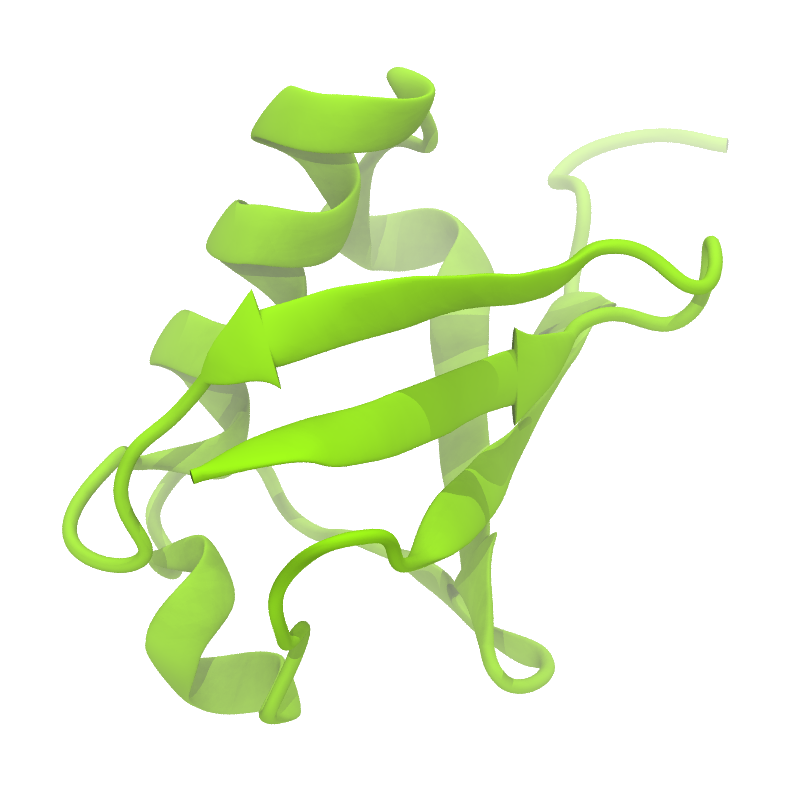 B
B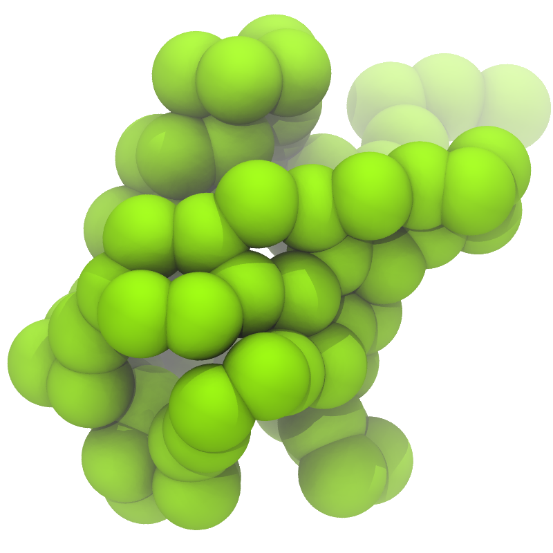 C
C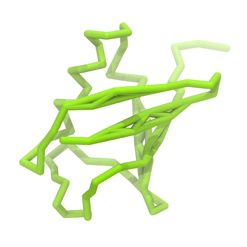
Figure 1 | Different representations of ubiquitin. A) cartoon representation of the atomistic structure. B) Coarse-grained beads forming the backbone and C) licorice representation of the backbone of the martinized protein.
4. Do a short (ca. 10 steps is enough!) minimization in vacuum. Before you can generate the input files with grompp, you will need to check that the topology file (.top) includes the correct martini parameter file (.itp). If this is not the case, change the include statement. Also, you may have to generate a box, specifing the dimensions of the system, for example using editconf. You want to make sure, the box dimensions are large enough to avoid close contacts between periodic images of the protein, but also to be considerably larger than twice the cut-off distance used in simulations. Try allowing for a minimum distance of 1 nm from the protein to any box edge. Then, copy the example parameter file, and change the relevant settings to do a minimization run. Now you are ready to do the preprocessing and minimization run:
$ editconf -f 1UBQ-CG.pdb -d 1.0 -o 1UBQ-CG.gro
$ grompp -f minimization-vaccum.mdp -p system-vaccum.top -c 1UBQ-CG.gro -o minimization-vaccum.tpr
$ mdrun -deffnm minimization-vaccum -v
5. Solvate the system with genbox (an equilibrated water box can be downloaded here; it is called water.gro, in the command below, it is saved as water-box-CG_303K-1bar.gro). Make sure the box size is large enough (i.e. there is enough water around the molecule to avoid periodic boundaries artifacts) and remember to use a larger van der Waals distance when solvating to avoid clashes, e.g.:
$ genbox -cp minimization-vaccum.gro -cs water-box-CG_303K-1bar.gro -vdwd 0.21 -o system-solvated.gro
6. Do a short energy minimization and position restrained simulation of the solvated system. Since the martinize.py script already generated position restraints (thanks to the -p flag), all you have to do is specify define = -DPOSRES in your parameter file (.mdp) and add the appropriate number of water beads (the molecule name is W) to your system topology (.top); the number can be seen in the output of the genbox command.
$ grompp -f minimization.mdp -c system-solvated.gro -p system.top -o minimization.tpr
$ mdrun -deffnm minimization -v
$ grompp -f equilibration.mdp -c minimization.gro -p system.top -o equilibration.tpr
$ mdrun -deffnm equilibration -v
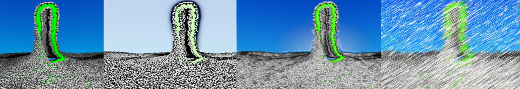
7. Start production run (without position restraints!); if your simulation crashes, some more equilibration steps might be needed. A sample trajectory is shown in Figure 2.
$ grompp -f dynamic.mdp -c equilibration.gro -p system.top -o dynamic.tpr
$ mdrun -deffnm dynamic -v
Figure 2 | 20 ns simulation of coarse-grained ubiquitin (green beads) and solvent (coarse-grained water; blue beads).
8. PROFIT! What sort of analysis can be done on this molecule? Start by having a look at the protein with vmd.
Soluble protein: the elastic network approach
Download all the files of this module
The aim of this second module is to see how application of elastic networks can be combined with the Martini model to conserve secondary, tertiary and quartenary structures more faithfully without sacrificing realistic dynamics of a protein. We offer two alternative routes. Please be advised that this is an active field of research and that there is as of yet no "gold standard". The first option is to generate a simple elastic network on the basis of a standard Martini topology. The second options is to use an ElNeDyn network. This second option constitutes quite some change to the Martini force field and thus is a different force field in itself. The advantage is that the behavior of the method has been well described[2]. Both approaches can be set up using the martinize.py script and will be shortly described below.
We recommend to simulate a pure Martini coarse-grained protein (without elastic network) in a first step, and then see what changes are observed when using an elastic network on the same protein. Note that you'll need to simulate the protein for tens to hundreds of nanoseconds to see major changes in the structure; sample simulations are provided in the archive.
Martini
1. Repeat steps 1 to 7 from the previous exercise with the HIV-1 protease (1A8G.pdb).
2. Visualize the simulation, look especially at the binding pocket of the protein: does it stay closed, open up? What happens to the overall protein structure?
Martini + elastic network
The first option to help preserve higher-order structure of proteins is to add to the standard Martini topology extra harmonic bonds between non-bonded beads based on a distance cut-off. Note that in standard Martini, long harmonic bonds are already used to impose the secondary structure of extended elements (sheets) of the protein. The martinize.py script will generate harmonic bonds between backbone beads if the options -elastic is set. It is possible to tune the elastic bonds (e.g.: make the force constant distance dependent, change upper and lower distance cut-off, etc.) in order to make the protein behave properly. The only way to find the proper parameters is to try different options and compare the behavior of your protein to an atomistic simulation or experimental data (NMR, etc.). Here we will use basic parameters in order to show
the principle.
1. Use the martinize.py script to generate the coarse-grained structure and topology as above. For the elastic network, use the extra following flags:
$ martinize.py [...] -elastic -ef 500 -el 0.5 -eu 0.9 -ea 0 -ep 0
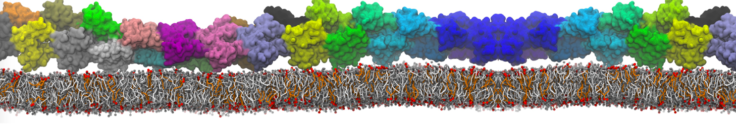
This turns on the elastic network (-elastic), sets the elastic bond force constant to 500 kJ.mol-1.nm-2 (-ef 500), the lower and upper elastic bond cut-off to 0.5 and 0.9 nm, respectively (-el 0.5 and -eu 0.9), and makes the bond strengths independent of the bond length (elastic bond decay factor and decay power, -ea 0 and -ep 0, respectively; these are default). The elastic network is defined in the .itp file by an #ifdef statement, and is switched on by default (#define NO_RUBBER_BANDS in the .top or .itp file switches it off). Note that martinize.py does not generate elastic bonds between i → i+1 and i → i+2 backbone bonds, as those are already connected by bonds and angles (cf. Fig. 3).
Figure 3 | Elastic network (gray) applied on the both monomer of the HIV-1 protease (yellow and orange, respectively)
2. Proceed as before (steps 4 to 7) and start a production run. Keep in mind we are adding a supplementary level of constraints on the protein; some supplementary relaxation step might be required (equilibration with position restraints and smaller time step for instance).
ElNeDyn
The second option to use elastic networks in combination with Martini puts more emphasis on remaining close to the overall structure as deposited in the PDB than standard Martini does. The main difference from the standard way (used in the previous exercise) is the use of a global elastic network between the backbone beads to conserve the conformation instead of relying on the angle/dihedral potentials and/or local elastic bonds to do the job. The position of the backbone beads is also slightly different: in standard Martini the center of mass of the peptide plane is used as the location of the backbone bead; but in the ElNeDyn implementation the positions of the Cα-atoms are used instead. The martinize.py script automatically sets these options and sets the correct parameters for the elastic network. As the elastic bond strength and the upper cut-off have to be tuned in an ElNeDyn network, these options can be set manually (-ef and -eu flags); note however these parameters have been extensively studied and were optimized to 500 kJ.mol-1.nm-2 and 0.9 nm[2].
1. Use the martinize.py script to generate the coarse-grained structure and topology as above. The following flag will switch martinize.py to the ElNeDyn default representation:
$ martinize.py [...] -ff elnedyn22
2. Proceed as before and start a production run.
Now you've got three simulations of the same protein with different type of elastic networks. If you do not want to wait, some pre-run trajectories can be found in the archive. One of them might fit your needs in terms of structural and dynamic behavior. If not, there are an almost infinite number of ways to further tweak the elastic network!
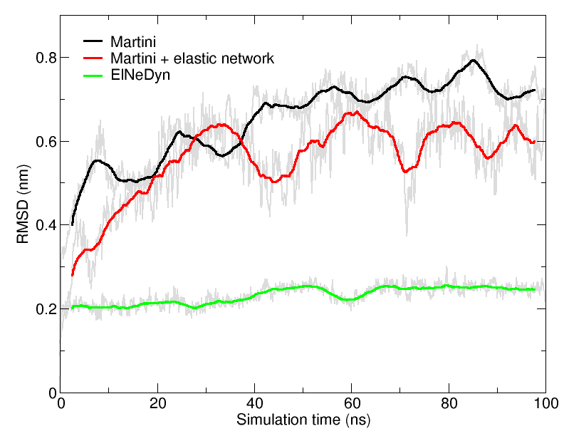
Figure 4 | RMSD of HIV-1 protease backbone with the three different approaches described previously (RMSD is usually considered "reasonnable" if below 0.3 nm).
An easy way to compare the slightly different behaviors of the proteins in the previous three cases is to follow deviation/fluctuation of the backbone during simulation (and compare it to an all-atom simulation if possible). RMSD (Fig. 4) and RMSF can be calculated using gromacs tools. vmd provides also a set of friendly tools to compute these quantities, but needs some tricks to be adapted to coarse-grained systems (standard keywords are not understood by vmd on coarse-grained structures).
To go further: membrane protein
Download all the files of this module (worked with old-style lipid collection topology file)
Download the minimum set of files for this module and set everything up yourself using the lipidome topologies
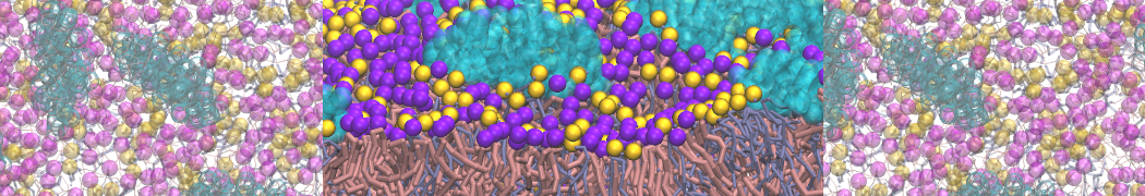
In the last module of this protein tutorial, we will increase the complexity of our system by embedding the protein in a lipid bilayer (the tutorial on old-style lipid bilayer can be followed here and the tutorial using the lipidome is here). We propose here to have a look at the tilt and the dimerization of KALP peptides embedded in DPPC membrane. The coarse-grained structure (kalp.gro) and topology (kalp.itp) of KALP are given in the archive; no need to repeat steps 1 to 4 martinizing the peptide from above. We will start here from step 5 since we are going to use a different way of solvating the proteins. Many different options to perform this step are available to us; a non-exhaustive list, ordered by decreasing complexity, is presented below:
- A bilayer self-assembly dynamic, as presented in the first module of the lipid tutorial, will result in the self-insertion of the WALP inside the bilayer (Fig. 5).
A
B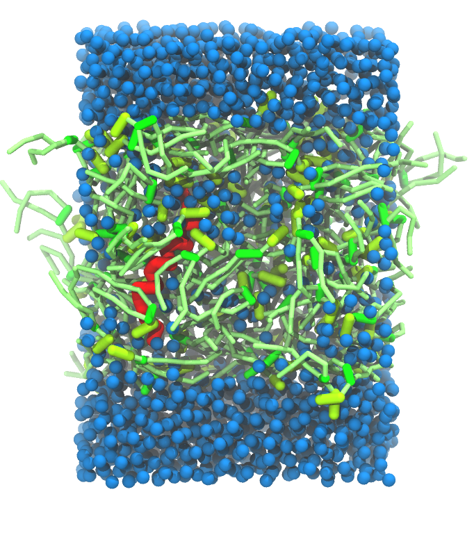 C
C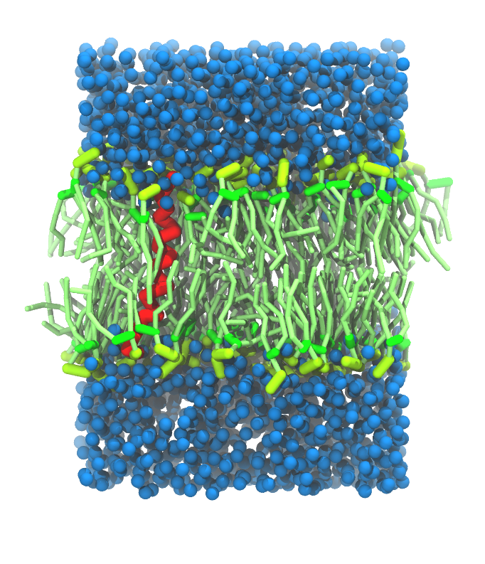
Figure 5 | A) Self-assembly (4 ns) of a DPPC (green) bilayer embedding a KALP peptide. B) Initial "soup" of lipid and solvent (water; blue) in which the KALP (red) is mixed. C) Final conformation of the simulation.
- If a stable DPPC membrane with the wanted box dimensions is already available, genbox will be able to insert the peptides in the bilayer (the peptides have to be pre-centered and positioned to ensure their presence inside the membrane).
- The use of the script insane.py, downloadable here.
The latter allows the insertion of a protein in a bilayer with any composition. Being the easiest and the most straightforward, we recommend this way of doing and that is what we are presenting here.
1. The syntax of the insane.py scripts is very similar to what was used so far; it can be invoked by running insane.py -h. Let's see a practical example:
$ insane.py -f kalp.gro -o system.gro -p system.top -pbc square -box 10,10,10 -l DPPC -center -sol W
The previous command line will set up a complete system, containing a squared DPPC bilayer of 10 nm, insert the KALP peptide centered in this bilayer and solvate the whole thing in standard coarse-grained water. More on the insane.py tool can be found in separate tutorials, notably setting up a complex bilayer. (with old-style lipids here).
2. Proceed as before and start a production run. To remind you, this involves (1) editing the system.top file to reflect the version of Martini you want to use (the KALP topology provided is version 2.1) and providing include statements for the topology files; (2) downloading or copying definitions of Martini version you want and the DPPC lipid topology file from the lipidome; (3) using the correct names of the molecules involved; (4) downloading or copying set-up .mdp files for minimization, equilibration, and production runs and if necessary, editing them (bilayer simulations are best done using semi-isotropic pressure coupling and you may want to separately couple different groups to the thermostat(s)); (5) running the minimization and equilibration runs.
3. Generate a new system in which membrane thickness is reduced (different the lipid type, DLPC for instance). Observe how the thickness is affecting the tilt of the transmembrane helix; compare it to the previous simulation.
4. Double these previous boxes in one dimension (genconf) and rerun the simulations. Observe the different dimerization conformations (parallel or anti-parallel tilts). Note that more than one simulation might be required to observe both cases!
5. Choose your favorite orientation and reverse-map the last conformation (tutorial on reverse-mapping available here). Simulate this system atomistically to refine and have a closer and detailed look at the interactions between KALPs.
Tools and scripts used in this tutorial
gromacs (http://www.gromacs.org/)
martinize.py (downloadable here)
insane.py (downloadable here)
[1] L. Monticelli, S.K. Kandasamy, X. Periole, R.G. Larson, D.P. Tieleman, S.J. Marrink. The MARTINI coarse grained forcefield: extension to proteins. J. Chem. Theory Comput., 4:819-834, 2008.
[2] X. Periole, M. Cavalli, S.J. Marrink, M.A. Ceruso. Combining an elastic network with a coarse-grained molecular force field: structure, dynamics, and intermolecular recognition. J. Chem. Theory Comput., 5:2531-2543, 2009.
Martini tutorial: reverse-mapping
- Details
-
Last Updated: Monday, 23 August 2021 10:31
Other tutorials
Backward
The method
Mapping
Backmapping aquaporin 1
Reverse transformation
Polarizable water
CHARMM-GUI Martini Maker
Backward
Backmapping or reverse coarse-graining or fine-graining a coarse-grained (CG) structure requires a correspondence between the two models; i.e., for atomistic and CG: which atoms make up which bead. Actually, an atom can in principle contribute to several beads. A backmapping protocol needs to know at least which atoms contribute to which bead. Existing schemes then use rigid building blocks anchored on the CG bead, or place the atoms randomly near the bead in an initial guess and the structure is relaxed based on the atomistic force field, usually by switching it on gradually. The method used in this tutorial is baskward[1], developed by Tsjerk Wassenaar. Bakwards allows for an intelligent, yet flexible initial placement of the atoms based on the positions of several beads, thereby automatically generating a very reasonable orientation of the groups of atoms with respect to each other.
First, we go over the scripts used in the backward[1] method. Second, we describe the structure and setup of the needed CG to fine-grained mapping files, taking the mapping file for valine as an example. Last, we demonstrate the method by backmapping a CG membrane embedded aquaporin 1, as described in[2].
More extensive discussion and examples, including tutorial material can be found in the paper by Wassenaar et al.[1], and Supporting Material to that paper.
The method
The backward program is available here, and consists of three scripts and a number of CG to fine-grained mapping definition files. The scripts are backward.py, initram.sh and the Mapping directory __init__.py and a number of .map files. The .map files describe the CG to fine-grained mapping and a file needs to be provided for each molecule (or it’s building blocks) in your system. The __init__.py script interprets the .map files. The backward.py script performs the actual backmapping and initram.sh is a bash wrapper that runs a series of minimizations and molecular dynamics steps, using the fine-grained force field to push the initial backmapped structure to one that satisfies the fine-grained force field.
Mapping
A requirement for the procedure to work is that the subdirectory Mapping contains definitions for how the atomic positions are generated from the CG positions. The subdirectory Mapping contains a file for each residue and/or molecule that can be backmapped, named for the atomistic target force field, e.g. val.oplsaa.map for a valine residue targeted to OPLS-AA. The structure of a .map file is explained below for the valine residue. The file val.oplsaa.map reads:
[ molecule ]
VAL
[ martini ]
BB SC1
[ mapping ]
oplsaa
[ atoms ]
1 N BB
2 H BB
3 CA BB
4 HA BB
5 CB SC1 BB
6 HB SC1 BB
8 CG1 SC1
9 HG11 SC1
10 HG12 SC1
11 HG13 SC1
12 CG2 SC1
13 HG21 SC1
14 HG22 SC1
15 HG23 SC1
16 C BB
17 O BB
[ chiral ]
CB CA N C
HB CA N C
[ chiral ]
HA CA N CB C ;L-Val
;HA CA N C CB ;D-Val
[ out ]
CG2 CB CG1 CA
HG21 CB CG1 CA
HG22 CB CG1 CA
HG23 CB CG1 CA
Directives analogous to gromacs topologies contain specifications that build the atomistic structure from the CG positions. The [ molecule ] directive contains the name of the residue or molecule. The [ martini ] directive contains the names of the CG beads in the Martini model: valine has two beads called BB and SC1. The [ mapping ] directive contains the name of the object model. Note that this directive may contain multiple object models. If you do not care for the naming convention of different force fields, you can use the same mapping file for the CHARMM36 and OPLS-AA/L force fields, because these are both all-atom models which in the GROMACS implementation also use the same order of the atoms (if not the same names). Thus, the mapping files for the methylated terminal ends explicitly state that they can be used for mapping to both OPLS-AA and CHARMM36 force fields.
The [ atoms ] directive contains the index numbers and names of the atoms in the object model and their relation to the CG beads. Note that a single atom may be in a relation with more than one CG bead. The back-mapping procedure starts by putting each atom that is related to a single bead on the position of that bead. If an atom is related to more than one bead, it will be placed on the weighted average position of the beads listed. It is allowed to list the same bead multiple times; thus the line
4 OE1 BB BB BB SC1 SC1
places the fourth atom (with name OE1) of the residue on the line connecting the BB and SC1 beads at 2/5 of the distance between the beads, starting at the BB bead. This mechanism is a simple aid to position atoms already at fairly reasonable starting positions. Using the -kick flag displaces all atoms randomly after their initial placement. Note that the script applies a random kick to atoms that are initially put at exactly the same place, e.g. because they are defined by the position of a single bead. Thus, no two atoms will be on top of each other. Switching on an atomistic force field usually results in an error if two interacting atoms are at exactly the same place.
The backward procedure implements a few other more sophisticated mechanisms to place atoms and some are used in the valine residue. Implementation can be found in the file Mapping/__init__.py. The [ chiral ] directive generates stereochemically specifically arranged groups of atoms. As is seen for valine, two types of input can be provided. In the first instance of the [ chiral ] directive, four atoms are listed on a line. The first atom is the atom to be placed (named A in Figure 1e, chiral*) on the basis of the positions of the other three. The Figure shows how vectors are defined from the positions of the other three particles to construct the position of the first atom. In the second instance of the [ chiral ] directive, five atoms are listed on a line. This corresponds to the construction shown in Figure 1d, chiral. The [ out ] directive may be used to spread out several equivalent atoms (as on a CH3-group) away from the center of the bead in a reasonable manner, as shown in Figure 1c, out. Again, be aware that atoms initially placed on the same spot, are randomly displaced; therefore, using the same reference atoms as in the example still leads to different positions for the generated atoms.
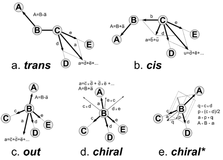
Figure 1 | Figure from[1]. Prescriptions for placing atom A on the basis of the positions of other atoms (upper case letters B, C, D, E). The other atoms define vectors (lower case letters a, b, c, d, e, p, q) that are used to calculate the position of A. A bar is used over the vectors to denote their normalization. The x denotes taking the outer product of two vectors.
Backmapping aquaporin 1
Here we backmapp a CG membrane embedded aquaporin 1 into CHARMM36 atomistic coordinates, as described in[2]. The files for this part of the tutorial are available in aquaporine_backmap.zip. Missing residues were added to aquaporin 1 and it was converted to Martini CG coordinates, solvated in a CG POPC bilayer with ions and polarizable water. Then simulated for 100 ns at the CG level with position restrains on the protein, see[2] for method details and CG_posre.gro for final coordinates. Note, without position restrains on the protein the CG protein might (depending on the protein in question and the CG force field used) evolve to far away from a possible fine-grained structure, rendering backmapping impossible.
We are going to use the initram.sh script, which calls backward.py and then runs a series of minimization and equilibrium simulations to get the final backmapped structure. To run the script we need the following:
The CG structure to backmapp, provided in CG_posre.gro
A complete fine-grained force field corresponding to all the CG molecules in CG_posre.gro. Here we use CHARMM36, see all .itp files provided and topol.top, which contains the molecules in the same order they are present in CG_posre.gro and with the same names. Note, water and ions can be skipped in the .top files as they are automatically detected by backward.py.
A .map file in the Mapping directory for all residues and molecules to be backmapped (water and ions can also be skipped here as their definitions are included in backward.py).
The initram.sh script uses the gromacs package so a proper version needs to be sourced.
Run the script using the following command:
$ ./initram.sh -f CG_posre.gro -o aa_charmm.gro -to charmm36 -p topol.top
After successful backmapping the aa_charmm.gro file will contain POPC membrane embedded aquaporin 1 as well as the solvent at fully atomistic resolution according to the CHARMM36 force field. Figure 2 illustrates the backmapping of a few POPC molecules. When running the backmapping script please keep in mind that initram.sh generates a significant number of temporary files so backmapping in a separate directory can be a good idea and that backward.py used random kicks to initially displace the atoms so rerunning the same command can give different results (and even though some runs might results in an error others may not).
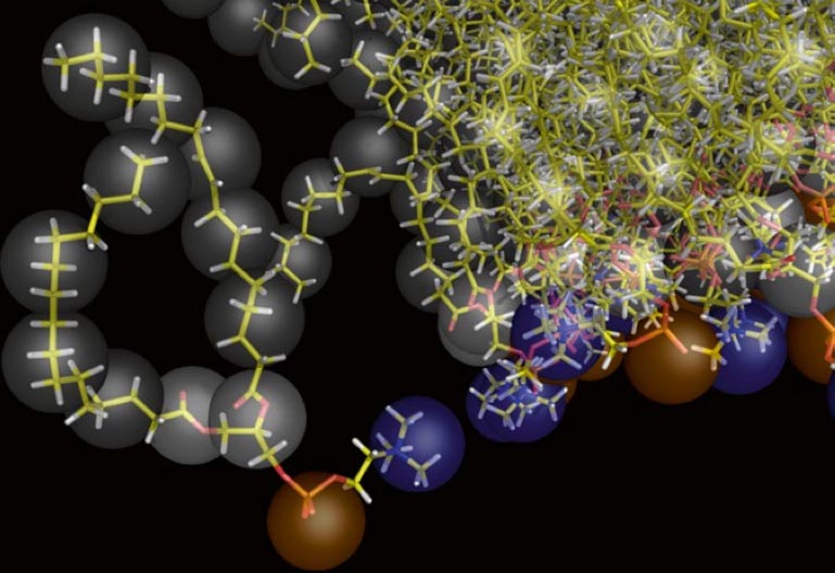
Figure 2 | Backmapped all-atom representation of a Martini POPC membrane. Figure from[2].
Reverse transformation
In this module we explore the use of the reverse-transformation tool, to convert between coarse-grained and fine-grained representations of a system.
Simulations at coarse-grained level allow the exploration of longer time-scales and larger length-scales than at the usual atomistic level. However, the loss of detail can seriously limit the questions that can be asked to the system. Methods that re-introduce atomic details in a CG structure are therefore of considerable interest. Such structures provide starting points in phase space for simulations at the more detailed level that may otherwise take too long to reach. As a demonstration of such a method, we will use restrained simulated annealing (SA) to increase the resolution of a system containing a WALP peptide spanning a DPPC bilayer. We will investigate how the number of steps allowed for the reconstruction influences the quality of the generated FG structure.
Reverse transformation: transformation run
In this part of exercise we will use a modi�ed version of gromacs that allows one to generate a FG structure from CG beads[3]. The same version is also used to transform a FG structure to CG beads, section 1e. Thus, the program allows one to switch between FG and CG representations. To achieve this, additional information is put in the topology �le at the FG level in a section called [ mapping ]. The tool pdb2gmx can generate this mapping for proteins automatically. Note that this will usually require the option -missing to be speci�ed! Two new functions in mdrun are responsible for restrained simulated annealing (SA) to converge from a random FG structure to a FG structure compatible with the CG structure, i.e. the FG positions are optimized in such a way that the CG structure is preserved in the FG-to-CG mapping (each CG bead is at the center of mass of the FG atoms that map to it). There is also small tool, called g_fg2cg, to generate CG structures from FG ones defi�ned by the mapping and random FG starting structures based on CG input �le, that are afterwards optimized during a SA run.
The source code for this version of the script can be found Downloads/Tools section of this website.
The files needed for this section can be downloaded from: rev_trans.tar.gz
Transformation run
1. Unpack the rev_trans.tar.gz in the MARTINITUTORIAL directory that contains all necessary gromacs �files for this exercise.
2. Compile and/or source the modifi�ed version of gromacs (remember this tool is based upon gromacs version 3.3.1 and needs the corresponding tricks and threats to be compiled.)
$ source /where-ever-you-installed-it/gromacs-3.3.1/bin/GMXRC
$ export GMXLIB=/where-ever-you-installed-it/gromacs-3.3.1/share/gromacs/top
3. Modify the FG fg.top fi�le in such a way that the number of water and lipid molecules is the same as in the coarse-grained model. One FG_W corresponds to four normal water molecules.
4. Use g_fg2cg to construct an input atomistic structure for a simulated annealing run. The coarse grain structure is already prepared for you and is called cg.gro. Check the output with ngmx or VMD.
$ g_fg2cg -pfg fg.top -pcg dppc_cg.top -n 0 -c cg.gro -o fg.gro
5. Use grompp to create a topol.tpr �file.
6. Perform a SA run by typing
$ mdrun -coarse cg.gro -v
7. Change the number of simulation steps to 1000 and SA time parameters to 0 1.5 0 1.5 0 1.5 in your .mdp file. (see comments for additional .mdp options at the bottom of fg.mdp �file) Perform another SA run with the altered parameters.
8. Change the number of simulation steps to 5000 and SA time parameters to 0 7.5 0 7.5 0 7.5. Perform a SA run again.
9. If you have enough time, change the number of simulation steps to 60000 and SA time parameters to 0 100 0 100 0 100. Repeat the SA run.
10. Plot the potential energies for all runs and compare them.
11. Compare FG WALP models from all runs. Check secondary structure and phi� and psi angles.
12. Compare dihedral distribution for one of dihedral angles from the tail of the DOPC lipids.
Polarizable water
In this part of the tutorial we will convert water in an existing Martini-system to polarizable water. In the polarizable Martini paper[4] the model is described as follows:
"The polarizable CG water consists of three particles instead of one in the standard Martini force �eld. The central particle W is neutral and interacts with other particles in the system by means of the Lennard-Jones interactions, just like the standard water particle. The additional particles WP and WM are bound to the central particle and carry a positive and negative charge of +0.46 and -0.46, respectively. They interact with other particles via a Coulomb function only, and lack any LJ interactions. The bonds W-WP and W-WM are constrained to a distance of 0.14 nm. The interactions between WP and WM particles inside the same CG water bead are excluded, thus these particles are "transparent" toward each other. As a result the charged particles can rotate around the W particle. A harmonic angle potential with equilibrium angle phi = 0 rad and force constant Kh = 4.2 kJ mol-1 rad-2 is furthermore added to control the rotation of WP and WM particles and thus to adjust the distribution of the dipole momentum."
If you want to solvate a new system with polarizable water, follow the steps in the lipid or protein Martini tutorials. Instead of a normal waterbox and .mdp/.itp fi�les use the waterbox containing polarizable water and polarizable Martini .mdp and .itp fi�les (available from the Martini website: cgmartini.nl). Note that minimizing a polarizable Martini system requires some tweaking, as described below.
If you have an existing system with normal Martini water and want to change to polarizable water you may use the python script triple-w.py. For this example we convert dppc_bilayer.gro/dppc_bilayer.top available here.
1. Create a new gro �file:
$ triple-w.py dppc_bilayer.gro
The python-script triple-w.py adds positive and negative sites at a small distance to every central water bead in a .gro �file.
2. Adapt the .top file. Make sure the polarizable version of the particle defi�nition martini_v2.P.itp fi�le is included. In the .mdp file the value of epsilon_rc has to be adapted and the index group W renamed into PW (Download an example here). The .itp �files for the lipids and possibly other molecules do not have to be changed.
3. If polarizable water is used in combination with proteins or peptides, all AC1 and AC2 beads have to be replaced by normal C1 and C2 beads. AC1 and AC2 are obsolete in polarizable Martini.
4. Minimize the system. For polarizable water to minimize without problems, it is SOMETIMES necessarry to change the constraints to stiff� bonds. Using the ifdef-statement in the martini_v2.P.itp fi�le, this can be set using a de�fine value in the .mdp fi�le (have a look at the bottom of martini_v2.P.itp to see how it works).
5. Set the correct options in martini_v2.P_example.mdp (e.g. "integrator = steep", "nsteps = 50", "constraints = none", "epsilon_r = 2.5", etc.) and the "defi�ne" option to -DEM and change the W index group name.
6. Generate the input fi�les for the minimization run:
$ grompp -f martini_v2.P_example.mdp -c dppc-polW.gro -p dppc bilayer.top -o em -maxwarn 1
7. Proceed with equilibration and production runs.
CHARMM-GUI Martini Maker
The CHARMM-GUI input generator now supports the Martini force field[5]. The Martini Maker supports building solution, micelle, bilayer, and vesicle systems, and systems with randomly distributed lipids. The Martini Maker has all the common Martini lipids as well as supporting variations of the Martini model (polar and nonpolar Martini, Dry Martini, and ElNeDyn). The CHARMM-GUI has an easy to use step-by-step user interface, please explore the Martini Maker input generator at http://www.charmm-gui.org/.
Following is a very short tutorial on how to make a Dry Martini vesicle using Martini Maker.
-
Go to the CHARMM-GUI -> Input Generator -> Martini Maker -> Vesicle Builder website.
-
Select the box for Vesicle Only System and in the drop-down menu, select the Dry Martini option, then press Next Step: Select Lipids.
-
Set the vesicle radius to 120 Å and generate a single-lipid system containing only DPPC lipids by setting the ratio of DPPC to 1, leaving the value for all other lipids to 0. Then press Next Step: Determine the System Size. The webserver will set to work and show you what it is doing. Wait for the process to finish.
-
In the Step1 menu, you will be given some information about the system. Add 150 mM NaCl ions (this is the default set for you). Then press Next Step: Build Components. Again, the server is working for you. Wait for the process to finish; this may take some time.
-
In the Step2 menu, just press Next Step: Assemble Components. The server is working for you. Wait for the process to finish. Note that references are made to ions and solvent. Since you have selected Dry Martini, not solvent will be added, but the server may still issue solvent-related comments.
-
You are still in the Step2 menu. Press Next Step: Assemble Components. More work is done by the server. Wait for the process to finish.
-
In the Step3 menu, information regarding the system size and contents is shown. Set the temperature to 323 K. Press Next Step: Generate Equilibration and Dynamics Inputs. The server works to provide you with gromacs files. These files are packed into an archive (charmm-gui.tgz). A download button for this archive is shown in red in the top right-hand side corner.
-
Download the final files and unpack them on your computer (tar -zxvf charmm-gui.tgz). The archive expands to a directory called charmm-gui. You will find the gromacs input files in the folder charmm-gui/gromacs/. Enter this folder.
-
The README file is helpful by showing you the commands for running the energy minimization and equilibrium steps using the provided .mdp files. Note that in gromacs 5 and above gromacs commands are not called directly but through gmx e.g. not grompp but gmx grompp (or gmx_d grompp). You may need to change that in the README file if you want to use it as a shell command that automatically executes the entire protocol.
-
Note, the vesicle equilibrium runs require gromacs version 5.1 or greater. In the equilibrium runs pores through the vesicle bilayer are held open to allow lipids to flop-flop and equilibrate between the inside/outside leaflets. The potentials used to keep those pores open are only supported in gromacs version 5.1 or greater. Pores are kept open using so-called flat-bottomed position restraints. These are described in the Version 5 manual in section 4.3.2. The pores are activated/controlled by setting the define = -DVESICLE_LIPIDTAIL_R=1 in the .mdp file. This flag activates position restraints set in the .itp of all the lipids and the provided restraint coordinates file lipidtail_posres.pdb.
-
Note, the initial energy minimization normally requires a double precision installation of gromacs. The reason is that some beads may be very close to each other in the initial structure, leading to very high forces; in the single-precision installation, these forces may be interpreted as infinite and therefore cause the minimization to fail. There is a workaround that problem, however. By using soft-core potentials in the first minization steps, forces will not be infinite and the double precision version is not required. The script equivalent to the README file containing the protocol and the setting .itp files for the dry DPPC vesicle of this tutorial are available here. Note that for other systems, you may need edits. After download, place the soft-core-minimization.tgz file in the folder charmm-gui/gromacs/. Unpack and run the protocol.
$ tar -xzvf soft-core-minimization.tgz
$ ./minimization-equilibration.sh
-
A word of WARNING! Proper equilibration of lipids between the leaflets, even with the open pores can take quite long, and will vary depending on vesicle size and lipids composition. The default time for the equilibrium runs is set to 500 ns which will take very long if run on your desktop machine.
The structure (.gro) files after each equilibration step and after the 1 µs simulation can be downloaded here.
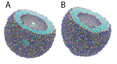
Figure 3 | DPPC Dry Martini vesicle with 5171 lipids. Part of the vesicle is cutoff to show inside. A) After energy minimization – showing x2 of the pores to equilibrate the leaflets. B) After 1 µs production simulation.
[1] Wassenaar, T. A., Pluhackova, K., Böckmann, R. A., Marrink, S. J., and Tieleman, D. P. (2014) Going Backward: A Flexible Geometric Approach to Reverse Transformation from Coarse Grained to Atomistic Models. J. Chem. Theory Comput. 10, 676–690.
[2] Pluhackova, K., Wassenaar, T. A., and Böckmann, R. A. (2013) Molecular Dynamics Simulations of Membrane Proteins, in Methods in Molecular Biology (Rapaport, D., and Herrmann, J. M., Eds.), pp 85–101. Humana Press.
[3]<Rzepiela, A. J., Schäfer, L. V., Goga, N., Risselada, H. J., De Vries, A. H., and Marrink, S. J. (2010) Reconstruction of atomistic details from coarse-grained structures. J. Comput. Chem. 31, 1333–1343.
[4] Yesylevskyy, S. O., Schäfer, L. V., Sengupta, D., and Marrink, S. J. (2010) Polarizable Water Model for the Coarse-Grained MARTINI Force Field. PLoS Comput Biol 6, e1000810
[5] Qi, Y., Ingólfsson, H.I., Cheng, X., Lee, J., Marrink, S.J., and Im, W. (2015) CHARMM-GUI Martini Maker for coarse-grained simulations with the Martini force field. JCTC, doi:10.1021/acs.jctc.5b00513.
Martini tutorial: DNA
- Details
-
Last Updated: Tuesday, 31 January 2017 14:10
Martini tutorials: DNA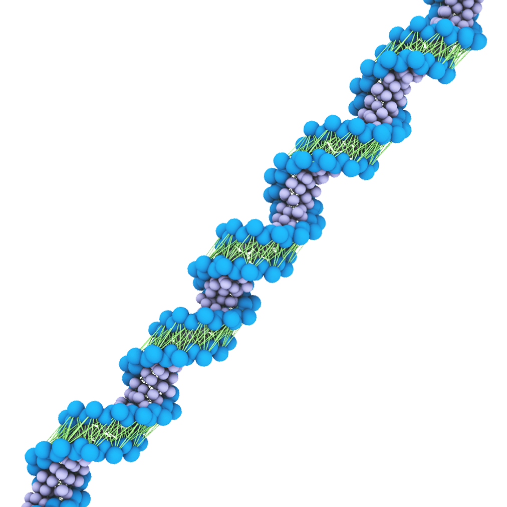
Contents
Basic system setup: Double stranded DNA
Debugging: Common problems
Case: Input from sequence
Analysis: Helical parameters
Persistence length
System setup: protein-DNA complex
Backmapping: DNA and Backwards
NOTE: You can download all the files required for this tutorial from here. Please note that you have to adjust some of the paths (mostly location of the force field files) below if you use this package.
Setting up double-stranded DNA
This is a brief tutorial on how to set up and try out DNA Martini simulations. To complete this tutorial you should download the latest Martini DNA release beta from here. It includes the itp files for DNA as well as a modified martinize script to coarse grain a DNA molecule.
Martini DNA can be used to model both single-stranded as well as double-stranded DNA and provides two separate elastic networks. This tutorial will show only an example of creating a dsDNA topology using the stiff elastic network but a dsDNA topology with soft network or a ssDNA topology without elastic network can be created using the same procedure. For dsDNA structures the stiff elastic network is a good starting point for seeing how your system behaves in a CG simulation. There are also options for creating elastic networks for more complicated DNA structure, martinize-dna optionsall-stiffandall-softare meant to be starting points for creating topologies for such structures but they are beyond the scope of this tutorial. The DNA release package intrjconv -s 03-run.tpr -f 03-run.xtc -o ../DNA_analysis/dna.xtc -pbc clustercludes a README file that should have sufficient instructions for creating the other types of DNA topologies after you have finished this tutorial.
1. Unpack the tutorial files you downloaded (it expands todna-tutorial).
$ tar -xvzf dna-tutorial.tgz
2. Go to the folder dna-tutorial/martini-dna and download the 1BNA PDB file if you didn't already. Martinize for DNA works best with cleaned up .gro files so you should first remove other atoms from the .pdb file and convert it to a .gro file.
$ grep -v HETATM 1BNA.pdb > 1BNA-cleaned.pdb
$ editconf -f 1BNA-cleaned.pdb -o 1BNA-cleaned.gro
3. Next we can use martinize-dna.py (supplied for you in the current directory) to create a Martini DNA topology for 1BNA.
$ python martinize-dna.py -dnatype ds-stiff -f 1BNA-cleaned.gro -o cg-dna.top -x cg-1bna.pdb
Next, you need to change the .top file to include the correct .itp files. This can be done with your favourite text editor but scriptable options are given below. Note: there are two sets of commands here, the first for Mac OSX, the second for Linux. In both cases, the backslashes (\) need to be typed as indicated.
OSX
$ sed -i .bak 's/#include "martini.itp"/#include "martini_v2.1-dna.itp"\
#include "martini_v2.0_ions.itp"/' cg-dna.top (OS X)
and Linux
$ cp cg-dna.top cg-dna.top.bak (Linux)
$ sed -i 's/#include "martini.itp"/#include "martini_v2.1-dna.itp"\n#include "martini_v2.0_ions.itp"/' cg-dna.top (Linux)
4. You can visualize the mapping of Martini DNA by opening both the atomistic and coarse-grained structures in VMD. (The visualization is clearer if you show the CG structure as small VDW spheres.)
$ vmd -m 1BNA-cleaned.pdb cg-1bna.pdb
5. Next you need to create a simulation box for DNA and solvate it as well as add counterions. (Download box of water from here.)
$ editconf -f cg-1bna.pdb -d 1.2 -bt dodecahedron -o box.gro
$ genbox -cp box.gro -cs water.gro -o bw.gro -vdwd 0.22 -maxsol 1250
You can replace water with ions in .top file without using genion at the same time as we add waters there. Note: the next line assumes that exactly 1250 water beads were added to the DNA by the genbox tool; the first 1100 added beads are designated as normal water beads, the next 128 beads are designated as anti-freeze water beads, and the final 22 beads are designated as sodium ions.
$ printf "\nW 1100\nWF 128\nNA 22\n" >> cg-dna.top
6. Use the example.mdp provided in the directory and make the required modifications to run an energy minimization (integrator = steep, nsteps = 100).
$ cp example.mdp example-em.mdp
$ [gedit/vi] example-em.mdp
$ grompp -f example-em.mdp -c bw.gro -p cg-dna.top -o 01-em -maxwarn 1
$ mdrun -v -deffnm 01-em
7. Next, you can run a short equilibration using the original example.mdp file. Note, a smaller time step might be needed for initial equilibration. If this is the case, edit the example.mdp file and specify a smaller time step. Do a series of short equilibrations, increasing the time step up to the value in the example.mdp file and starting each one from the final structure of the previous one.
$ grompp -f example.mdp -c 01-em.gro -p cg-dna.top -o 02-eq
$ mdrun -v -deffnm 02-eq -rdd 2.0
8. Now you are ready to start your first DNA simulation. Copy the example.mdp file to produce a longer simulation, do the preprocessing and start the simulation. Note that with the elastic network the domain cell size needs to be kept fairly large (option -rdd 2.0).
$ cp example.mdp example-run.mdp
$ [gedit/vi] example-run.mdp
$ grompp -f example-run.mdp -c 02-eq.gro -p cg-dna.top -o 03-run
$ mdrun -v -deffnm 03-run -rdd 2.0
9. You can visualize the movements of the DNA, ions and waters using VMD while your simulation is still running (you will need to open a new terminal). Note that bonds in Martini are longer than bonds normally shown in VMD. Please consult the VMD tutorial to get better visualization.
$ vmd 02-eq.gro 03-run.xtc
Common problems
Below are some some of the most common pitfalls when starting a Martini DNA simulation. We go through them here so that you know to avoid them when starting your own DNA simulations.
1. Not curating the input file formartinize-dna.py
There are several things that can go wrong beforemartinize-dna.pyis even run. Best course of action is to manually curate the input file, remove all heteroatoms and convert the file to a gro file.martinize-dna.pyrequires the residuenames to be 'DA','DC', etc. in order to detect them correctly.
You can try this yourself. Go to the foldercommon-problems/1inside the package you downloaded. Try runningmartinize-dna.pywith the given input file. Then try to fix the issue by modifying the residuenames using a text editor or a script (column editing in vi comes really handy here) and see thatmartinize-dna.pyruns succesfully after this.
2. Placing the "#define RUBBER_BANDS" below the DNA itp file in the system topology file.
The topology file is read from top to bottom and if theRUBBER_BANDSare not defined before the DNA itp file no elastic network will be applied to the DNA. This is the first place to look if the DNA structure is deforming right in the beginning of your simulation.
Go to the foldercommon-problems/2and run a short simulation with the provided files. Then open thecg.topfile and fix it and run the same simulation again and see the difference.
3. Getting wrong number of chains frommartinize-dna.py
This often goes unseen unless you check the output ofmartinize-dna.pyon your screen. Especially the 'Found X chains:...' part of the output. If a chain is split in two you can try to fix that by adjusting the cut-off inside the martinize-dna.py. Open the script and search forCUT-OFF_CHANGEand adjust the value from 3.0 to a suitably large value.
Go to the foldercommon-problems/3and open the gro file using VMD to see that the structure consist of 2 DNA strands. Next, try runningmartinize-dna.py(provided here in the same folder so you won't modify the version other parts of the tutorial use) on the given input file and verify from output that you get 3 chains instead of 2. Open martinize-dna.py with a text editor and search forCUT-OFF_CHANGEand adjust the cut-off value from3.0to4.0. Runmartinize-dna.pyagain and verify that it detects the DNA as 2 strands.
Input from sequence
In case you want to create an all-atom DNA structure from canonical values, there are several softwares/webservers that can help with this. One of those is NAFlex which requires only the user to create an account to save his/her projects. NAFlex allows several ways to build your DNA structure.
1. After giving a name for your project, we will select the option DNA/RNA Simulation from Sequence (although we will not run any simulation here).Click the "Next" button.
2. As an example you can build a relatively short oligonucleotide according to the right-handed B-DNA Arnott parameters with the following sequence (enter the string and click "Create Project":
ACAGCTAGCATGCATGCA
3.- Click on the "Next" buttons until you see a window with a pdb file (compare the picture below). Clicking on the link to the pdb file will reveal a set of buttons. Download the file. No it is time to check the output structure after you have downloaded and unzippid the output file.
4. You can now use the downloaded .pdb file and build a Martini model from it as shown for 1BNA in the previous section. You can copy the necessary files from that directory.
 #include "./tip3p.itp"
NB: NAFlex has multiple applications but in this tutorial we will focus on building a structure from ab initio.
DNA analysis: physical parameters
As for all-atomistic models, we can calculate the base pairs and base pair steps helical parameters for coarse-grained DNA models. cgHeliParm.py has been developed for the analysis of the DNA/RNA double stranded structures in molecular dynamics (MD) simulations. Like other atomistic softwares (e.g. 3DNA, Curves+), it defines a geometric reference frame for each base/base pair to calculate several structural descriptors of DNA/RNA from the GROMACS CG Martini MD trajectory. As output the helical descriptors as a function of time are saved in individual files.
For now, the current version of cgHeliParm.py allows to calculate the local structural parameters of double stranded DNA molecules (i.e. base pair and base pair step helical parameters). We are currently working on extending the calculation to other structural parameters such as groove dimensions. Please note that in this version only double-stranded, standard nucleic acids can be analysed. This excludes mispaired, modified, single-stranded DNA, triplexes and quadruplexes from its application.
Before using cgHeliParm.py you need first to install python in your computer. If you don’t have it, go to the Python wiki and follow the instructions to install it in your working computer.
The second thing you will have to do is to install the python package MDAnalysis. To install/upgrade it from the command line using easy_install or pip:
<p style="line-height: 1.38; margin-top: 0pt; margin-bottom: 0pt; text-align: justify;" dir="ltr"> </p>
easy_install -U MDAnalysis
pip install --upgrade MDAnalysis
R We have also included the MDAnalysis module called mdreader (thanks This email address is being protected from spambots. You need JavaScript enabled to view it.) to make the calculation more efficient and fast.
Once python and MDAnalysis package are installed and mdreader is in our working directory, we can use cgHeliParm.py. First, we will have to create a ‘dry’ trajectory with only DNA. This can be done using the trjconv Gromacs tool and the corresponding NDX file. For this case, we will use the same trajectory from the previous DNA tutorial (1BNA). Go to the martini-dna tutorial and convert the trajectory twice (selecting the group for DNA when prompted, which should be number 1).
trjconv -s 03-run.tpr -f 03-run.xtc -o ../DNA_analysis/dna.xtc -pbc cluster
trjconv -s 03-run.tpr -f 03-run.xtc -o ../DNA_analysis/dna.gro -dump 0
Now, change to the directory DNA_analysis:
cd ../DNA_analysis
in this directory, we can run the cgHeliParm.py script by running in the command line:
python cgHeliParm.py -f dna.xtc -s dna.gro -o dna
This may take some time depending on the length of your trajectory and number of processors available. After the script has finished you will see that there are several files in your folder, corresponding to base pair and base pair steps helical parameters (file names are informative). Each file contains information for each bp or step along the simulation time. The first column refers to the first bp or step in the 5’3’ strand sense.
Persistence length
We provide also a tool to calculate the persistence-length of a double-stranded DNA. This tool requires both a fairly long dsDNA strands as well as a long simulation so we provide an example trajectory to try this out. The tool uses two different ways of averaging the results but the numbers should be fairly close to each other.
To calculate the persistence length go to the folderpersistence-lengthand run the following command:
$ python persistence-length-calculator.py -s run.gro -f run.xtc -n run.ndx -oplot test -b 100000
Advanced tutorial: protein-DNA complex
DNA is recognized by proteins in many different ways. As a first approximation to protein-DNA complexes, we will use the SRY protein (1j46, which is provided in the directory, but can also be downloaded here), which is involved in sex determination, to generate our first protein-DNA complex simulation using the CG Martini model. Go to the directory dna-tutorial/protein_DNA.

First things first. To create our CG model of a protein-DNA complex from a PDB file we will need to split both protein and DNA molecules to generate their CG models. This means that you will need to create as many PDB files as molecules your complex has. To put everything on the same page, we will call them protein_AA.pdb and dna_AA.pdb. (This has been done for you already, you may want to also try it yourself!) We will then proceed to create their CG models with the corresponding martinize script.
1. We will first build the CG DNA using the martinize-dna script but before that we will convert the .pdb file into a .gro file:
editconf -f dna_AA.pdb -o dna_aa.gro
python martinize-dna.py -dnatype ds-stiff -f dna_aa.gro -o dna.top -x dna_CG.pdb
And for the CG protein model we will use the original martinize script:
editconf -f protein_AA.pdb -o protein_aa.gro
python martinize.py -f protein_aa.gro -o protein.top -x protein_CG.pdb -dssp /opt/local/bin/dssp -p backbone -ff elnedyn22
2. We will now merge the PDB files corresponding to the CG models (protein_CG.pdb and dna_CG.pdb) using the cat command for example.
cat dna_CG.pdb protein_CG.pdb > complex_CG.pdb
3. You can visualize the mapping of Martini DNA by opening both the atomistic and coarse-grained structures in VMD. The CG beads are best visualized as VDW spheres. Note that by concatenating the protein and DNA files, the combined CG coordinate file is interpreted by VMD as two frames. By stepping through them in the VMD main window, you can see the protein and the DNA sites.
vmd -m 1j46.pdb complex_CG.pdb
4. As in the double stranded DNA tutorial for 1BNA, we will create a .top file that includes the .itp files. We can copy the dna.top file and modify to include the correct .itp files. With the experience from previous tutorial, would you be able to write a .top file for the system yourself? Check by comparing your result to the provided file cg-complex.top.
5. Next we will solvate the solute creating a box around it as well as adding counterions. We will use the same water.gro file that we used previously to create the 1BNA CG model. (Download water box from here.) Note that by concatenating the protein and DNA files, the combined coordinate file is seen as two separate frames by GROMACS tools. Therefore, we need a preprocessing step.
grep ATOM complex_CG.pdb > complex_CG-cleaned.pdb
editconf -f complex_CG-cleaned.pdb -d 1.2 -bt dodecahedron -o box.gro
genbox -cp box.gro -cs water.gro -o bw.gro -vdwd 0.22 -maxsol 1250
You can replace water with ions in .top file without using genion at the same time as we add waters there.
printf "\nW 1100\nWF 124\nNA 26\n" >> cg-complex.top
6. Use the same example.mdp file provided with in the directory dna-tutorial/martini-dna and make the required modifications to run an energy minimization (integrator = steep, nsteps = 100).
grompp -f example-em.mdp -c bw.gro -p cg-complex.top -o 01-em -maxwarn 1
mdrun -v -deffnm 01-em
7. Next, you can run a short equilibration using the original example.mdp file. (Note, a smaller time step might be needed for initial equilibration).
grompp -f example.mdp -c 01-em.gro -p cg-complex.top -o 02-eq
mdrun -v -deffnm 02-eq -rdd 2.0
8. Now you are ready to start your first protein-DNA simulation. Modify the .mdp file to produce a longer simulation and start.
grompp -f example-run.mdp -c 02-eq.gro -p cg-complex.top -o 03-run
mdrun -v -deffnm 03-run -rdd 2.0
9. You can visualize the trajectory using VMD while your simulation is still running.
vmd 02-eq.gro 03-run.xtc
DNA and Backward
DNA structures can be backmapped into atomistic resolution using Backward. Before starting this part of the tutorial you should first go and do the Backward tutorial. The DNA backmapping files are as of now not yet part of the downloadable backward package but files for CHARMM are in the tutorial package in the backmapping folder together with the backward scripts. Next, we will first coarse-grain a dsDNA structure and then backmap it back to atomistic resolution.
1. Got to the dna-tutorial/backmapping directory and cleanup and convert the given DNA structure 1BNA.pdb to a gro file in a reasonable simulation box.
$ editconf -f 1BNA.pdb -d 1.4 -o 1BNA.gro
2. Create a CG structure using martinize-dna.py.
$ python ../martini-dna/martinize-dna.py -f 1BNA.gro -dnatype ds-stiff -p cg.top -x cg-1BNA.pdb
3. Solvate the CG structure.
$ genbox -cp cg-1BNA.pdb -cs waterbox.gro -vdwd 0.22 -o cg-1bna-water.gro
4. Create an atomistic topology file for the system. Choose charmm27 and tip3p when prompted.
$ pdb2gmx -f 1BNA.pdb
5. Edit the file topol.top to point explicitly to the tip3p.itp file provided for you (it will not recognize it in the standard path unfortunately). Thus, replace the line #include "charmm27/tip3p.itp" near the end of the file by #include "./tip3p.itp". Run the initram.sh script to perform the backmapping.
$ ./initram.sh -f cg-1bna-water.gro -o aa-charmm.gro -to charmm36 -p topol.top
6. Compare the initial structure to the backmapped structure.
$ vmd -m 1BNA.gro aa-charmm.gro
Martini tutorials: lipids
- Details
-
Last Updated: Thursday, 19 May 2016 15:05
Martini tutorials: lipids
Summary
Lipid bilayers
Bilayer self-assembly
Bilayer analysis
Area per lipid
Bilayer thickness
Lateral diffusion
Order parameters
Additional analysis
Changing lipid type
Complex bilayers
Advanced: Dry Martini and vesicles
Advanced: refine lipid parameters
Tools and scripts used in this tutorial
Next tutorial: Proteins
Lipid bilayers
The Martini course-grained (CG) model was originally developed for lipids[1,2]. The underlying philosophy of Martini is to build an extendable CG model based on simple modular building blocks and to use only few parameters and standard interaction potentials to maximise applicability and transferability. Martini uses an approximate 4:1 atomistic (heavy atoms) to CG bead mapping and in version 2.0[2] 18 bead types were defined to represent chemical characteristics of the beads. The CG beads have a fixed size and interact using an interaction map with 10 different interaction strengths. Due to the modularity of Martini, a large set of different lipid types has been parameterized e.g. the Martini lipid topology section.
These tutorials assume a basic understanding of the Linux operating system and the gromacs molecular dynamics (MD) simulation package. An excellent gromacs tutorial available at: md.chem.rug.nl/~mdcourse/.
The aim of the tutorial is to create and study properties of CG Martini models of lipid bilayer membranes. First, we will attempt to spontaneously self-assemble a DSPC bilayer and check various properties that characterize lipid bilayers, such as the area per lipid, bilayer thickness, order parameters, and diffusion. Next, we will change the nature of the lipid head groups and tails, and study how that influences the properties. Finally, we will move on to creating more complex multicomponent bilayers.
Download all the files of this tutorial: bilayer_tutorial.zip Unpack the lipid-tutorial.tar.gz archive (it expands to a directory called bilayer-tutorial).
Bilayer self-assembly
We will begin with self-assembling a distearoyl-phosphatidylcholine (DSPC) bilayer from a random configuration of lipids and water in the simulation box. Enter the spontaneous-assembly subdirectory; first, create a random configuration of 128 DSPC lipids starting from a single DSPC molecule:
$ genbox -ci dspc_single.gro -nmol 128 -box 7.5 7.5 7.5 -try 500 -o 128_noW.gro
Next, minimize the system...
$ grompp -f minimization.mdp -c 128_noW.gro -p dspc.top -maxwarn 10 -o dspc-min-init.tpr
$ mdrun -deffnm dspc-min-init -v -c 128_minimised.gro
...add 6 CG waters (i.e., 24 all-atom waters) per lipid...
$ genbox -cp 128_minimised.gro -cs water.gro -o waterbox.gro -maxsol 768 -vdwd 0.21
The value of the flag -vdwd (default van der Waals radii) has to be increased from its default atomistic length (0.105 nm) to a value reflecting the size of Martini CG beads.
...and minimize again (adapt dspc.top to reflect the water beads added to the system):
$ grompp -f minimization.mdp -c waterbox.gro -p dspc.top -maxwarn 10 -o dspc-min-solvent.tpr
$ mdrun -deffnm dspc-min-solvent -v -c minimised.gro
Now, you are ready to run the self-assembly MD simulation. About 25 ns should suffice.
$ grompp -f martini_md.mdp -c minimised.gro -p dspc.top -maxwarn 10 -o dspc-md.tpr
$ mdrun -deffnm dspc-md -v
This might take ca. 45 min on a single CPU but by default mdrun will use all available CPUs on your machine. You can tune the numbers of parallel threads mdrun uses with the -nt parameter. You may want to check the progress of the simulation to see whether the bilayer has already formed before the end of the simulation. You may do this most easily by starting the inbuilt gromacs viewer:
$ ngmx -f dspc-md.xtc -s dspc-md.tpr
or, alternatively, use VMD, the inital and final snapshots should look similar to Fig. 1. In the meantime, have a close look at the Martini parameter files; in particular, the interactions and bead types. What are the differences between PC and PE headgroups as well as between saturated and unsaturated tails?
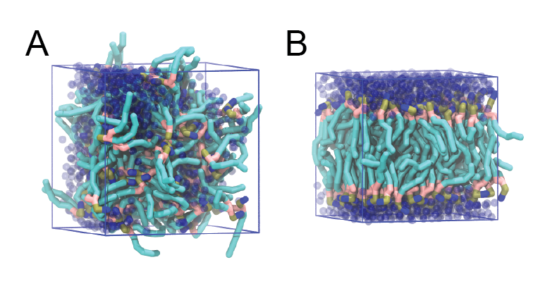
Figure 1 | DSPC bilayer formation. A) 64 randomly localized DSPC lipid molecules with water. B) After a 30 ns long simulation the DSPC lipids have aggregated together and formed a bilayer.
Check whether you got a bilayer. If yes, check if the formed membrane is normal to the z-axis (i.e., membrane in the xy-plane). If the latter is not the case, rotate the system accordingly (with editconf). In case you did not get a bilayer at all, continue with the pre-formed one from dspc_bilayer.gro. Set up a simulation for another 15 ns at zero surface tension (switch to semiisotropic pressure coupling) at a higher temperature of 341 K. This is above the experimental gel to liquid-crystalline transition temperature of DSPC. You will find how to change pressure coupling and temperature in the gromacs manual: manual.gromacs.org/current/online.html Again, you may not want to wait for this simulation to finish. In that case, you may skip ahead and use a trajectory provided in the subdirectory spontaneous-assembly/allfiles/.
Bilayer analysis
From the latter simulation, we can calculate properties such as:
- area per lipid
- bilayer thickness
- P2 order parameters of the bonds
- lateral diffusion of the lipids
In general, for the analysis, you might want to discard the first few ns of your simulation as equilibration time.
Area per lipid
To get the (projected) area per lipid, you can simply divide the area of your simulation box (Box-X times Box-Y from g_energy) by half the number of lipids in your system. (Note that this might not be strictly OK, because the self-assembled bilayer might be slightly asymmetric in terms of number of lipids per monolayer, i.e., the areas per lipid are different for the two monolayers. However, to a first approximation, we will ignore this here.)
Bilayer thickness
To get the bilayer thickness, use g_density. You can get the density for a number of different functional groups in the lipid (e.g., phosphate and ammonium headgroup beads, carbon tail beads, etc) by feeding an appropriate index-file to g_density (make one with make_ndx; you can select, e.g., the phosphate beads by typing a P*). The bilayer thickness you can obtain from the distance between the headgroup peaks in the density profile.
A more appropriate way to compare to experiment is to calculate the electron density profile. The g_density tool also provides this option. However, you need to supply the program with a data-file containing the number of electrons associated with each bead (option -ei electrons.dat). The format is described in the gromacs manual.
Compare your results to those from small-angle neutron scattering experiments[3]:
- thickness = 4.98 ± 0.15 nm
- area per lipid = 0.65 ± 0.05 nm2
Lateral diffusion
Before calculating the lateral diffusion, remove jumps over the box boundaries (trjconv -pbc nojump). Then, calculate the lateral diffusion using g_msd. Take care to remove the overall center of mass motion (-rmcomm*), and to fit the line only to the linear regime of the mean-square-displacement curve (-beginfit and -endfit options of g_msd). To get the lateral diffusion, choose the -lateral z option.
To compare the diffusion coefficient obtained from a Martini simulation to a measured one, a conversion factor of about 4 has to be applied to account for the faster diffusion at the CG level due to the smoothened free energy landscape (note, the conversion factor can vary significantly depending on the molecule in question).
*In gromacs v3, this option is not available. An additional trjconv -center will do the trick.
Order parameters
Now, we will calculate the (second-rank) order parameter, which is defined as:
P2 = 1/2 (3 cos2<θ> − 1),
where θ is the angle between the bond and the bilayer normal. P2 = 1 means perfect alignment with the bilayer normal, P2 = −0.5 anti-alignment, and P2 = 0 random orientation.
A script to calculated these order parameters can be downloaded here (there is also a version located in the directory scripts/). Copy the .xtc and .tpr files to a analysis subdirectory (the script expects them to be named traj.xtc and topol.tpr, respectively; you may want to use the 15 ns simulations already present in the subdirectory spontaneous-assembly/allfiles/). The script do-order-multi.py will calculate P2 for you. As it explains when you invoke it, it needs a number of arguments. The command:
$ ./do-order-multi.py traj.xtc 0 15000 20 0 0 1 64 DSPC
will for example read 0 to 15 ns from the trajectory traj.xtc. The simulation has 64 DSPC lipids and the output is the P2, calculated relative to the Z-axis, and average over results from every 20th equally-spaced snapshot in the trajectory.
Additional analysis
Different scientific questions require different methods of analysis and no set of tools can span them all. There are various tools available in the gromacs package, see the gromacs manual: manual.gromacs.org/current/online.html. Most simulation groups, therefore, develop sets of customized scripts and programs many of which they make freely available, such as the Morphological Image Analysis and the 3D pressure field tools available here. Additionally a number of packages are available to for assistance with analysis and the development of customized tools, such as the python MDAnalysis package pypi.python.org/pypi/MDAnalysis/.
Changing lipid type
Lipids can be thought of as modular molecules. In this section, we investigate the effect of changes in the lipid tails and in the headgroups on the properties of lipid bilayers using the Martini model. We will i) introduce a double bond in the lipid tails, and ii) change the lipid headgroups from phosphatidylcholine (PC) to phosphatidylethanolamine (PE).
Unsaturated tails
To introduce a double bond in the tail, we will replace the DSPC lipids by DOPC (compare the Martini topologies of these two lipids - martini_v2.0_lipids.itp). Replace DSPC by DOPC in your .top and .mdp files, and grompp will do the rest for you (you can ignore the ”atom name does not match” warnings of grompp).
Changing the headgroups
Starting again from the final snapshot of the DSPC simulation, change the head groups from PC to PE. For both new systems, run 15 ns MD simulations and compare the above properties (area per lipid, thickness, order parameter, diffusion) between the three bilayers (DSPC, DOPC, DSPE). Do the observed changes match your expectations? Why/why not? Discuss.
Complex bilayer mixtures
When setting up larger and more complex bilayers it can be more convenient, or necessary, to start with a bilayer close to equilibrium rather then trying to get the bilayer to self-assemble. This can be done by concatenating (e.g. using editconf) and/or altering previously formed bilayers or by using a bilayer formation program such as insane.py, available in the directory scripts/ or downloadable here. INSANE (INSert membrANE) is a CG building tool that generates membranes by distributing lipids over a grid. Lipid structures are derived from simple template definitions that can either be added to the program or provided on-the-fly from combinations of headgroup, linker and lipid tails specified on the command-line. The program uses two grids, one for the inner and one for the outer leaflet, and distributes the lipids randomly over the grid cells with numbers according to the relative quantities specified. This allows for building asymmetric bilayers with specific lipid compositions. The program also allows for adding solvent and ions, using a similar grid protocol it distributes them over a 3D grid. Additional information about the functionality of INSANE can be found by running insane.py -h.
In the directory complex-bilayers/ we will create a fully hydrated 4:3:3 mole ratio bilayer of DPPC:DUPC:CHOL with physiological ion concentration using insane.py, this is a similar mixture as was used in Risselada and Marrink[4] to show raft formation. Start by running INSANE:
$ ./insane.py -l DPPC:4 -l DUPC:3 -l CHOL:3 -salt 0.15 -x 15 -y 10 -z 9 -d 0 -pbc cubic -sol W -o dppc-dupc-chol-insane.gro
This will generate an initial configuration for the system dppc-dupc-chol-insane.gro (Fig. 2A) and provide initial information of the .top file. Next, fix the .top file by including the correct Martini topologies. Then, energy minimize the structure and run a short (10 ns) equilibrium simulation in a similar manner as explained in the bilayer self-assembly section. Note, as this simulation contains multiple components you will have to make an index file (using make_ndx) and group all the lipids together and all the solvent together to fit the specified groups in the .mdp files. As all the bilayer lipids and solvent were places on a grid (Fig. 2A), even after minimization they can still be in an energetically unfavorable state. Due to the large forces involved it may be necessary to run a few equilibrium simulations using a short time step (1-10 fs) before running production simulations with Martini lipid time steps (30-40 fs). The initial grid order imposed by insane.py should relax in a few ns (Fig. 2B), we recommend simulating for 5-30 ns using the Berendsen pressure coupling algorithm, to relax the membrane area, before switching to Parrinello-Rahman for the production run. This mixture will phase separate at a temperature of 295 K but that can take multiple microseconds (Fig. 2C).
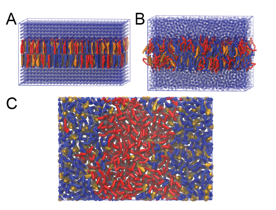
Figure 2 | DPPC-DUPC-CHOL bilayer formation. A) Using insane.py a 4:3:3 DPPC-DUPC-CHOL bilayer was setup. B) After a 20 ns long simulation the grid structure is gone and the bilayer area has equilibrated. C) This lipid mixture phase separates into Ld and Lo domains at 295 K, this phase separation can take multiple microseconds, showing a top view of the simulation after 6 microseconds. In all panels DPPC is in red, DUPC in blue and cholesterol in orange.
Advanced: Dry Martini and vesicles
In this tutorial we are going to study the deformation of a lipid vesicle due to demixing and formation of Lo and Ld phases. To study this type of system composed of a very large number of particles, a specific force field has recently been developed: Dry Martini. This Martini-derived force field, as its name indicates, doesn't require any aqueous solvent and allows the simulation of much larger systems.
The use of this force field requires very specific parameters for production runs; everything is explained in the package found there.
Update: We recommend that you generate your vesicle using the CHARMM-GUI. Follow the tutorial on how to use it here and continue to follow this tutorial after you've equilibrated your vesicle.
-
Generate the vesicle using the martini_vesicle_builder.py script available there. The following command will generate a 25 nm diameter vesicle with randomly distributed DPPC, DUPC (DLiPC) and cholesterol molecules.
$ python martini_vesicle_builder.py 12.5 DPPC:DUPC,60:40 43 1> system.gro 2> system.top
-
Minimize the system.
-
Equilibrate the system. In this case, a long equilibration is required: the vesicle is built based on properties (thickness and area per lipid) extracted from pure flat bilayers; these properties will be drastically modified by the curvature of the vesicle bilayer. Pores will form in the bilayer, but will be quickly closed and help the equilibration (lipid flip-flop) of the vesicle.
-
Production run should be at least 10 µs. Check the evolution of the geometry of the system: how is the demixing affecting the sphericity of the vesicle? An example is given in Figure 3.
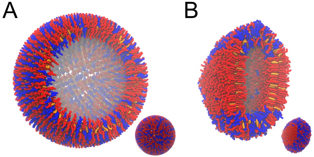
Figure 3 | DPPC-DUPC-CHOL vesicle, ball-to-doughnut transformation. A) Initial system, and B) conformation after a 20 µs long simulation: note the flatten sides of the vesicle, denoting the Lo phases (DPPC/CHOL). The insets are showing the full system, while the bigger snapshots are showing a cut.
Advanced: refine lipid parameters
Warning this section is a few years old and has not been tested recently. Also, this section uses the fine-grained-to-coarse-grained (FG-to-CG) transformation tool, which is treated in a later section of the Martini tutorial. If you are unfamiliar with the tool, you might want to skip this section.
In this part, we will try to obtain improved Martini parameters for diC18:2-PC, a PC lipid with a doubly unsaturated tail. We will try to optimise the Martini parameters such that the dihedral and angle distributions within the lipid tail match those from a 100 ns all-atom simulation (all-atom data in fg.xtc) as close as possible. The files needed in this section are located in the refine/ directory.
The task can be divided into the following five steps:
- Transform the all-atom (fine-grained, FG) trajectory into its coarse-grained counterpart, based on a pre-defined mapping scheme*.
- Calculate the angle and dihedral distributions. These will serve as the reference (“gold standard”) later.
- Do a coarse-grained simulation of the system.
- Calculate the angle and dihedral distibutions, and compare to the reference.
- Revise coarse-grained parameters, repeat steps 3 and 4 until you are satisfied with the result.
*The mapping is already defined, look at the [mapping] section in dupc_fg.itp.
For the transformation from FG to CG, we will use the program g_fg2cg, which is part of a modified version of gromacs that you need to install yourself (see tutorial "Reverse transformation"):
$ source /where-ever-your-installation-is/bin/GMXRC
$ setenv GMXLIB /where-ever-your-installation-is/share/top
First, transform from FG to CG:
$ g_fg2cg -pfg fg.top -pcg cg.top -c fg.gro -n 1 -o cg.gro
$ g_fg2cg -pfg fg.top -pcg cg.top -c fg.xtc -n 1 -o fg2cg.xtc
Then, make an index file needed for the calculation of the angle and dihedral distributions within the lipid tail:
$ make_ndx -f cg.gro -o angle.ndx
aGL1 | aC1A | aD2A
aC1A | aD2A | aD3A
aD2A | aD3A | aC4A
aC1A | aD2A | aD3A | aC4A
q
Now, calculate the distributions with g_angle:
$ g_angle -f fg2cg.xtc -type angle -n angle.ndx -od fg2cg ang{1,2,3}.xvg
$ g_angle -f fg2cg.xtc -type dihedral -n angle.ndx -od fg2cg dih1.xvg
These are the target distributions that we want to obtain with the CG model. As a starting point, we will use the Martini parameters as defined in dupc_cg.itp, i.e., all angles at 180 degrees. Carry out a short CG simulation (starting from cg_mdstart.gro, you just have to add water to the cg.top). (Don't forget to source a regular version of gromacs!) You will need to make an appropriate .mdp. Note that the FG trajectory was obtained at a temperature of 300 K. After comparing the angle and dihedral distributions to the g_fg2cg reference, change the angle parameters in dupc_cg.itp and repeat.
Tools and scripts used in this tutorial
gromacs (http://www.gromacs.org/)
insane.py (downloadable here)
MDAnalysis package (pypi.python.org/pypi/MDAnalysis/0.8.1)
[1] Marrink, S. J., De Vries, A. H., and Mark, A. E. (2004) Coarse grained model for semiquantitative lipid simulations. J. Phys. Chem. B 108, 750–760.
[2] Marrink, S. J., Risselada, H. J., Yefimov, S., Tieleman, D. P., and De Vries, A. H. (2007) The MARTINI force field: coarse grained model for biomolecular simulations. J. Phys. Chem. B 111, 7812–7824.
[3] Balgavy, P., Dubnicková, M., Kucerka, N., Kiselev, M. A., Yaradaikin, S. P., and Uhrikova, D. (2001) Bilayer thickness and lipid interface area in unilamellar extruded 1,2-diacylphosphatidylcholine liposomes: a small-angle neutron scattering study. Biochim. Biophys. Acta 1512, 40–52.
[4] Risselada, H. J., and Marrink, S. J. (2008) The molecular face of lipid rafts in model membranes. Proc. Natl. Acad. Sci. U.S.A. 105, 17367–17372.
Martini tutorials: lipids with lipidome
- Details
-
Last Updated: Thursday, 11 October 2018 13:01
Martini tutorials: lipids with the lipidome
Summary
Lipid bilayers
Bilayer self-assembly
Bilayer analysis
Area per lipid
Bilayer thickness
Lateral diffusion
Order parameters
Additional analysis
Changing lipid type
Complex bilayers
Advanced: refine lipid parameters
Tools and scripts used in this tutorial
Next tutorial: Proteins
Lipid bilayers
The Martini coarse-grained (CG) model was originally developed for lipids[1,2]. The underlying philosophy of Martini is to build an extendable CG model based on simple modular building blocks and to use only few parameters and standard interaction potentials to maximise applicability and transferability. Martini uses an approximate 4:1 atomistic (heavy atoms) to CG bead mapping and in version 2.0[2] 18 bead types were defined to represent chemical characteristics of the beads. The CG beads have a fixed size and interact using an interaction map with 10 different interaction strengths. Due to the modularity of Martini, a large set of different lipid types has been parameterized. Their parameters are available in the Martini Lipidome, see the Martini lipid topology section. In this tutorial, you will learn how to set up lipid-water system simulations with the lipidome, with a focus on bilayers. You will also study a number of standard bilayer properties.
These tutorials assume a basic understanding of the Linux operating system and the gromacs molecular dynamics (MD) simulation package. An excellent gromacs tutorial is available at: cgmartini.nl/~mdcourse/.
The aim of the tutorial is to create and study properties of CG Martini models of lipid bilayer membranes. First, we will attempt to spontaneously self-assemble a DPPC bilayer and check various properties that characterize lipid bilayers, such as the area per lipid, bilayer thickness, order parameters, and diffusion. Next, we will change the nature of the lipid head groups and tails, and study how that influences the properties. Finally, we will move on to creating more complex multicomponent bilayers.
Download all the files of this tutorial: bilayer_lipidome_tutorial.tgz Unpack the lipidome-tutorial.tgz archive (it expands to a directory called bilayer-lipidome-tutorial), and enter the bilayer-lipidome-tutorial directory:
$ tar -xzvf bilayer_lipidome_tutorial.tgz
$ cd bilayer-lipidome-tutorial
Bilayer self-assembly
We will begin with self-assembling a dipalmitoyl-phosphatidylcholine (DPPC) bilayer from a random configuration of lipids and water in the simulation box. Enter the spontaneous-assembly subdirectory. The first step is to create a simulation box containing a random configuration of 128 DPPC lipids. This can be done by starting from a file containing a single DPPC molecule. A file with coordinates for a single DPPC molecule is available for you as dppc_single.gro. The gromacs tool genbox can take this single-molecule conformation and attempt to place it in a simulation box multiple times at a random position and random orientation, each time checking that there are no overlaps between the consecutively placed molecules.
$ genbox -ci dppc_single.gro -nmol 128 -box 7.5 7.5 7.5 -try 500 -o 128_noW.gro
Perform a short energy minimization of the system containing only the lipids; the only reason for doing this, is getting rid of high forces between beads that may have been placed quite close to each other. The settings file minimization.mdp is provided for you, but you will need the topology for the DPPC lipid. Download it from the Martini lipidome page, see the Martini lipid topology section, place it in your current working directory, and check that the file name corresponds to the #include statement in the topology file dppc.top.
$ grompp -f minimization.mdp -c 128_noW.gro -p dppc.top -o dppc-min-init.tpr
$ mdrun -deffnm dppc-min-init -v -c 128_minimized.gro
Using the gromacs tool genbox again, add 6 CG waters (note that this corresponds to 24 all-atom waters) per lipid.
$ genbox -cp 128_minimized.gro -cs water.gro -o waterbox.gro -maxsol 768 -vdwd 0.21
The value of the flag -vdwd (default van der Waals radii) has to be increased from its default atomistic length (0.105 nm) to a value reflecting the size of Martini CG beads. The water beads are taken from the file water.gro provided for you. A new file, waterbox.gro is produced containing the 128 lipids and added water beads.
Now perform an energy minimization again. You will need to adapt dppc.top to reflect the water (W) beads added to the system. Look at the output of genbox to see how many W beads were added; the maximum number is 768 (specified on the last command as the -maxsol option). Remember that in gromacs files a semicolon (;) preceeds a comment line and is not interpreted as input!
$ [gedit/vi/other editor] dppc.top
$ grompp -f minimization.mdp -c waterbox.gro -p dppc.top -o dppc-min-solvent.tpr
$ mdrun -deffnm dppc-min-solvent -v -c minimized.gro
Now, you are ready to run the self-assembly MD simulation. About 30 ns should suffice.
$ grompp -f martini_md.mdp -c minimized.gro -p dppc.top -o dppc-md.tpr
$ mdrun -deffnm dppc-md -v
This might take approximately 45 minutes on a single CPU but by default mdrun will use all available CPUs on your machine. You can tune the numbers of parallel threads mdrun uses with the -nt parameter. You may want to check the progress of the simulation to see whether the bilayer has already formed before the end of the simulation. You may do this most easily by starting the inbuilt gromacs viewer (you will need to open a new terminal and make sure you are in the directory where this simulation is running):
$ ngmx -f dppc-md.xtc -s dppc-md.tpr
or, alternatively, use VMD or pymol. Both VMD and pymol suffer from the fact that Martini bonds are usually not drawn because they are much longer than standard bonds and the default visualization is not very informative. For visualization with pymol this is solved most easily by converting the trajectory to .pdb format, explicitly writing out all bonds. The disadvantage is that very large files are produced in this conversion!
$ trjconv -s dppc-md.tpr -f dppc-md.xtc -o dppc-md.pdb -pbc whole -conect
$ pymol dppc-md.pdb
For VMD, a plugin script cg_bonds.tcl was written that takes the Gromacs topology file and adds the Martini bonds defined in the topology. In general, a useful preprocessing step for VMD visualization is to avoid molecules being split over the periodic boundary, because if they are, very long bonds will be drawn between them. A script do_vmd.sh has been prepared for you for visualization using VMD. To learn more about visualizing Martini systems using VMD, consult the VMD tutorial.
$ ./do_vmd.sh
The inital and final snapshots should look similar to Fig. 1, at least if the self assembly resulted in a bilayer in the alloted time, which is not guaranteed.
In the meantime, have a close look at the Martini parameter files. The available bead types and their interactions are defined in the file martini_v2.1.itp. This file contains the definitions of version 2.1, and also includes the definition of the water bead, right at the bottom of the file. The lipid DPPC is defined in the file martini_v2.0_DPPC_01.itp , which you downloaded from the lipidome page. Get out the 2007 Martini paper[2] and check the definition of this molecule. Understanding how these files work, will help you work with the Martini model and define new molecules or refine existing models.
Figure 1 | DPPC bilayer formation. A) 64 randomly localized DPPC lipid molecules with water. B) After a 30 ns long simulation the DPPC lipids have aggregated together and formed a bilayer.
When the simulation has finished, check whether you got a bilayer. If yes, check if the formed membrane is normal to the z-axis (i.e., that the membrane is situated in the xy-plane). Have a look at the self-assembly process: can you recognize intermediate states, such as micelles, and do you see metastable structures such as a water pore and/or a lipid bridge?
Bilayer equilibrium run and analysis
If your bilayer was formed in a plane other than the xy-plane, rotate the system so that it will (with editconf). In case you did not get a bilayer at all, you can continue the tutorial with the pre-formed one from dspc-bilayer.gro. From this point on, we will refer to the bilayer as a DSPC bilayer. In Martini, the 4-to-1 mapping limits the resolution and the same model represents in this case a C-16 tail (palmitoyl) and a C-18 tail (stearoyl, hence DSPC). The reason for referring to the lipid as DSPC is that later on, we will compare the simulated properties to experiment and we will compare different lipids all with the same number of beads, changing either the head group from PC to PE or changing the tail from stearoyl (C-18, fully saturated) to oleoyl (C-18, single cis double bond at C-9).
The spontaneous assembly simulation was done using isotropic pressure coupling. The bilayer may have formed but is probably under tension because of the isotropic pressure coupling. Therefore, we first need to run a simulation in which the area of the bilayer can reach a proper equilibrium value. This requires that we use independent pressure coupling in the plane and perpendicular to the plane. Set up a simulation for another 30 ns at zero surface tension (switch to semiisotropic pressure coupling; if the pressure is the same in the plane and perpendicular to the plane, the bilayer will be at zero surface tension) at a higher temperature of 341 K. This is above the experimental gel to liquid-crystalline transition temperature of DSPC. You will find how to change pressure coupling and temperature in the gromacs manual: manual.gromacs.org/current/online/mdp_opt.html Again, you may not want to wait for this simulation to finish. In that case, you may skip ahead and use a trajectory provided in the subdirectory spontaneous-assembly/equilibration/.
From the latter simulation, we can calculate properties such as:
- area per lipid
- bilayer thickness
- P2 order parameters of the bonds
- lateral diffusion of the lipids
In general, for the analysis, you might want to discard the first few ns of your simulation as equilibration time. The area per lipid as a function of time should give you an indication of which part of the simulation you should definitely not include in the analysis.
Area per lipid
To get the (projected) area per lipid, you can simply divide the area of your simulation box by half the number of lipids in your system. The box-sizes can be obtained by running the gromacs tool g_energy (ask for Box-X and Box-Y). Then either use awk or xmgrace to calculate the area per lipid as a function of time. The gromacs tool g_analyze provides a convenient way to calculate the average and error estimate in any series of measurements (use the option -ee for the error estimate, and make sure you feed g_analyze a file with a .xvg extension). (Note that this calculation might not be strictly OK, because the self-assembled bilayer might be slightly asymmetric in terms of number of lipids per monolayer, i.e., the areas per lipid are different for the two monolayers. However, to a first approximation, we will ignore this here.)
Bilayer thickness
To get the bilayer thickness, use g_density. You can get the density for a number of different functional groups in the lipid (e.g., phosphate and ammonium headgroup beads, carbon tail beads, etc) by feeding an appropriate index-file to g_density (make one with make_ndx; you can select, e.g., the phosphate beads by typing a P*). The bilayer thickness you can obtain from the distance between the headgroup peaks in the density profile.
A more appropriate way to compare to experiment is to calculate the electron density profile. The g_density tool also provides this option. However, you need to supply the program with a data-file containing the number of electrons associated with each bead (option -ei electrons.dat). The format is described in the gromacs manual.
Compare your results to those from small-angle neutron scattering experiments[3]:
- thickness = 4.98 ± 0.15 nm
- area per lipid = 0.65 ± 0.05 nm2
Lateral diffusion
Before calculating the lateral diffusion, remove jumps over the box boundaries (trjconv -pbc nojump). Then, calculate the lateral diffusion using g_msd. Take care to remove the overall center of mass motion (-rmcomm*), and to fit the line only to the linear regime of the mean-square-displacement curve (-beginfit and -endfit options of g_msd). To get the lateral diffusion, choose the -lateral z option.
To compare the diffusion coefficient obtained from a Martini simulation to a measured one, a conversion factor of about 4 has to be applied to account for the faster diffusion at the CG level due to the smoothened free energy landscape (note, the conversion factor can vary significantly depending on the molecule in question).
*In gromacs v3, this option is not available. An additional trjconv -center will do the trick.
Order parameters
Now, we will calculate the (second-rank) order parameter, which is defined as:
P2 = 1/2 (3 cos2<θ> − 1),
where θ is the angle between the bond and the bilayer normal. P2 = 1 means perfect alignment with the bilayer normal, P2 = −0.5 anti-alignment, and P2 = 0 random orientation.
A script to calculated these order parameters can be downloaded here (there is also a version located in the directory scripts/). Copy the .xtc and .tpr files to a analysis subdirectory (the script expects them to be named traj.xtc and topol.tpr, respectively; you may want to use the 30 ns simulations already present in the subdirectory spontaneous-assembly/equilibration/). The script do-order.py will calculate P2 for you. As it explains when you invoke it, it needs a number of arguments. The command:
$ ./do-order.py my.xtc my.tpr 15000 30000 20 0 0 1 128 DPPC
will for example read 15 to 30 ns from the trajectory my.xtc. The simulation has 128 DPPC lipids and the output is the P2, calculated relative to the Z-axis, and average over results from every 20th equally-spaced snapshot in the trajectory. (Remember, DSPC and DPPC share the same Martini representation!)
Advanced: additional analysis
Different scientific questions require different methods of analysis and no set of tools can span them all. There are various tools available in the gromacs package, see the gromacs manual: manual.gromacs.org/current/online.html. Most simulation groups, therefore, develop sets of customized scripts and programs many of which they make freely available, such as the Morphological Image Analysis and the 3D pressure field tools available here. Additionally a number of packages are available to for assistance with analysis and the development of customized tools, such as the python MDAnalysis package pypi.python.org/pypi/MDAnalysis/.
Changing lipid type
Lipids can be thought of as modular molecules. In this section, we investigate the effect of changes in the lipid tails and in the headgroups on the properties of lipid bilayers using the Martini model. We will i) introduce a double bond in the lipid tails, and ii) change the lipid headgroups from phosphatidylcholine (PC) to phosphatidylethanolamine (PE).
Unsaturated tails
To introduce a double bond in the tail, we will replace the DSPC lipids by DOPC. Set up a directory for the DOPC system. Enter that directory. Download the topology for DOPC from the Martini lipidome web page. Compare the Martini topologies of these two lipids. You will see that the number of beads for these lipids is the same. You can therefore set up a DOPC bilayer quite simply from your DSPC result. Copy over the .top and .mdp file from the equilibration DSPC run. Copy the final frame of the DSPC run to serve as the starting frame of the DOPC run. Replace DPPC by DOPC in your .top and .mdp files, and grompp will do the rest for you (you can ignore the ”atom name does not match” warnings of grompp). Execute the simulation, or - if you are impatient - use the trajectory provided for you as spontaneous-assembly/equilibration/dopc/dopc-ext.xtc. NOTE: because the lipids DSPC and DOPC have exactly the same number of beads, you can use the .tpr file from DSPC to analyze the dopc-ext.xtc file.
Changing the headgroups
Similarly, starting again from the final snapshot of the DSPC simulation, you can easily change the head groups from PC to PE. Download the topology for DPPE from the Martini lipidome web page. Also for this system, run a 30 ns MD simulation, or - if you are impatient - use the trajectory provided for you as spontaneous-assembly/equilibration/dspe/dspe-ext.xtc. NOTE: because the lipids DSPC and DOPC have exactly the same number of beads, you can use the .tpr file from DSPC to analyze the dopc-ext.xtc file.
Compare the above properties (area per lipid, thickness, order parameter, diffusion) between the three bilayers (DSPC, DOPC, DSPE). Do the observed changes match your expectations? Why/why not? Discuss.
Complex bilayer mixtures
When setting up larger and more complex bilayers it can be more convenient, or necessary, to start with a bilayer close to equilibrium rather then trying to get the bilayer to self-assemble. This can be done by concatenating (e.g. using editconf) and/or altering previously formed bilayers or by using a bilayer formation program such as insane.py, available in the directory scripts/ or downloadable here. INSANE (INSert membrANE) is a CG building tool that generates membranes by distributing lipids over a grid. Lipid structures are derived from simple template definitions that can either be added to the program or provided on-the-fly from combinations of headgroup, linker and lipid tails specified on the command-line. The program uses two grids, one for the inner and one for the outer leaflet, and distributes the lipids randomly over the grid cells with numbers according to the relative quantities specified. This allows for building asymmetric bilayers with specific lipid compositions. The program also allows for adding solvent and ions, using a similar grid protocol it distributes them over a 3D grid. Additional information about the functionality of INSANE can be found by running insane.py -h.
In the directory complex-bilayers/ we will create a fully hydrated 4:3:3 mole ratio bilayer of DPPC:DIPC:CHOL with physiological ion concentration using insane.py, this is a similar mixture as was used in Risselada and Marrink[4] to show raft formation. The lipid DIPC is representative for tails containing two cis-unsaturated bonds and of length 16-18 carbons. Start by running INSANE (downloaded or copied from the scripts/ directory):
$ python insane.py -l DPPC:4 -l DIPC:3 -l CHOL:3 -salt 0.15 -x 15 -y 10 -z 9 -d 0 -pbc cubic -sol W -o dppc-dipc-chol-insane.gro
This will generate an initial configuration for the system dppc-dipc-chol-insane.gro (Fig. 2A). Download the relevant lipid topologies from the Martin lipdome and provide this information together with the system composition to the .top file. (Check that the file provided for you is correct.)
Then, energy minimize the structure and gently equilibrate the system. Note, as this simulation contains multiple components you will have to make an index file (using make_ndx) and group all the lipids together and all the solvent together to fit the specified groups in the .mdp files; the .mdp files provided expect the names Lipids and Solvent. As all the bilayer lipids and solvent were placed on a grid (Fig. 2A), even after minimization they can still be in an energetically unfavorable state. Due to the large forces involved it may be necessary to run a few equilibrium simulations using a short time step (1-10 fs) before running production simulations with Martini lipid time steps (30-40 fs). The initial grid order imposed by insane.py should relax in a few ns (Fig. 2B), we recommend simulating for 5-30 ns using the Berendsen pressure coupling algorithm, to relax the membrane area, before switching to Parrinello-Rahman for the production run. This mixture will phase separate at a temperature of 295 K but that can take multiple microseconds (Fig. 2C). A sample run is provided for you in the directory bilayer-lipidome-tutorial/complex-bilayers/raftmix.xtc. The INSANE script can also be used to set up a complex (or simple!) bilayer system including membrane protein, see the Martini protein tutorial.
Figure 2 | DPPC-DIPC-CHOL bilayer formation. A) Using insane.py a 4:3:3 DPPC-DIPC-CHOL bilayer was setup. B) After a 20 ns long simulation the grid structure is gone and the bilayer area has equilibrated. C) This lipid mixture phase separates into Ld and Lo domains at 295 K, this phase separation can take multiple microseconds, showing a top view of the simulation after 6 microseconds. In all panels DPPC is in red, DIPC in blue and cholesterol in orange.
Advanced: refine lipid parameters
This section uses the backward.py tool for fine-grained-to-coarse-grained (FG-to-CG) transformation, which is treated in more detail elsewhere. A related, but different strategy not using the backward.py tool is used in the tutorial on polymers, advantageous there because the PEG molecule is simpler to map from FG to CG representation than lipids.
In this part, we will outline how atomistic simulations can be used to obtain improved Martini parameters for selected degrees of freedom. You may then take this strategy to whatever lengths you deem fit. Remember, Martini in general does not aim to be specific for one particular molecule, but recognizes that the four-to-one mapping results in Martini molecules being representative of several closely related molecules. However, you may want to develop a specific model or compare how well Martini covers closely related molecules.
Here, we study diC18:2-PC, a PC lipid with a doubly unsaturated tail, in the Martini lipidome denoted as DIPC. Specifically, the atomistic (FG) model is for dilineoylphosphatidylcholine. The lineoyl tail is fully denoted as C18:2c9,12. This notation shows that the tail is 18 carbons long (counting starts at the ester C-atom, bound to the two O-atoms), contains two cis bonds, starting at carbon 9 and carbon 12, respectively (i.e. the cis-bonds are between carbons 9-10 and 12-13). We will show how to compare distributions of selected angles between beads for a mapped FG model to those from a Martini simulation. You can then use the distributions to guess and refine selected Martini parameters such that the distributions match those from the FG simulation as close as possible. The files needed in this section are located in the bilayer-lipidome-tutorial/refine/ directory. The FG trajectory is in fg.xtc. This contains only the lipids from a simulation of a lipid bilayer consisting of 128 lipids (64 per monolayer) in water.
The task can be divided into the following five steps:
- Transform the all-atom (fine-grained, FG) trajectory into its coarse-grained counterpart, based on a pre-defined mapping scheme.
- Calculate selected angle distributions. These will serve as the reference (“gold standard”) later.
- Do a coarse-grained simulation of the system.
- Calculate the selected angle distibutions, and compare to the reference.
- Revise coarse-grained parameters, repeat steps 3 and 4 until you are satisfied with the result.
For the transformation from FG to CG, we will use the tool backward.py, which is described in more detail elsewhere. You do not need to download this tool; it is provided in the refine/ directory. The refine/Mapping directory contains a file dipc.gromos.map that defines the mapping from the FG to the CG model. Have a look at it. You will see how each (united) atom of the FG lipid contributes to a CG bead. The order of the CG beads in the CG model is provided under the [ martini ] directive. Beads will appear in the output file in this order. It is important that this order corresponds to your proposed Martini model. Check the correspondence by inspecting the file refine/martini_v2.0_DIPC.itp. This contains the proposed Martini model. If you wish to alter the mapping scheme, you can do so by assigning the atoms differently to the beads. In general, we aim to adapt the mapping such that we get predominantly unimodal distributions for bonds and angles; however, we also want to stay within the Martini scheme of 4-to-1 mapping and mapping to recognizable chemical groups. As long as you can rationalize your choices, Martini is quite flexible.
1. Transformation of the FG trajectory to a mapped CG trajectory
Backward.py can perform the mapping from the FG to the CG model for .pdb and .gro files, but not (yet) for entire trajectories. Thus, the FG trajectory is first written out in single frames, and each frame is mapped from FG to CG using backward.py. When all CG frames are done, they are concatenated into a single CG trajectory - the time stamp is lost in this process! The mapping procedure is done for you in the bash script do-mapping.sh. Please inspect it before you execute it. Before you do the mapping, you need to have a .tpr file for the FG system.
$ grompp -p system.top -c lipid.gro -f min.mdp -o fg.tpr -maxwarn 10
$ ./do-mapping.sh
You will see that two directories have been created: FRAMES contains all the FG frames dumped from the trajectory; CGFRAMES contains all the CG frames converted from the FG frames and the mapped trajectory (CGFRAMES/cg-mapped.xtc).
2. Calculation of the selected angle distributions
Angle distributions can be calculated using the gromacs tool g_angle. This requires an index file containing multples of three indices. The three indices are the atoms/beads that define an angle. In this case, you have 128 lipids that each contain one or more angles you are interested in. You want to pool the data from equivalent angles and collected over the entire trajectory. This is best done by calculating the angle of interest for each lipid as a function of time, collect all equivalent angle data in one file and generate a distribution from that data. The bash script angledistr.sh does that for you. However, before you start, you need to provide a list of angles you are interested in. The script expects a file called anglelist containing one or more lines consisting of three numbers. The numbers are the indices of the angle(s) of interest. The numbers refer to a single lipid. The script will convert these for each lipid individually, depending on the number of lipids and the number of beads of each lipid. You may need to change these variables (NMOL and NAT, respectively) in the script. You can also adapt the script to take data from only a subset of the lipids, for example to calculate error bars on your distributions. Now, start the script or take a look at the files first and then start the script.
$ [ gedit/vi ] anglelist
$ [ gedit/vi ] angledistr.sh
$ ./angledistr.sh
You will see that a new directory has been created: ANGLES contains all data of all the angles of all the lipids as a function of time (cga_n.m.xvg), numbering the angles (n) and lipids (m) from 0 onward. Angle 0 corresponds to the first angle in the file anglelist. The distribution of the pooled data for each angle in the file anglelist can be found in the file ANGLES/cga_n-distr.xvg, where n is a number. You may inspect these files using a plot program, e.g. xmgrace. If all is well, the four angle distributions should look like those given in the files cfMappedAngleDistributions.agr, and cfMappedAngleDistributions.png.
These are the target distributions that we want to obtain with the CG model.
3. CG simulation
As a starting point, go to the directory refine/take0. We will use the Martini parameters as defined in martini_v2.0_DIPC.itp, i.e., the angles for the angles around the double-bond beads are defined with the minimum energy at 120 degrees. Carry out a short CG simulation (starting from cg_mdstart.gro).
$ grompp -p cg.top -c cg_mdstart.gro -n run.ndx -f martini_md.mdp -o cg.tpr
$ mdrun -deffnm cg
Alternatively, you may want an educated guess based on the distributions before you start out on take0. There is a tool to help you. Go back to the directory refine. The python script do_fit.py fits harmonic or periodic potentials to target distributions and returns parameters for the reference length or angle and force constant. NOTE: you will need to have the python package symfit installed! As an example, try the first angle:
$ python do_fit.py -f ANGLES/cga_0-distr.xvg -x0 100 -k 25 --harmonic --radians
You will see a window with the target distribution in blue and the first guess gaussian distribution in red. On the bottom of the window are sliders; you can adjust them to give a better fit. The parameter values will serve as the starting values of a best fit. Closing this window triggers the fitting procedure to start, and will result in best fit parameters and a new window showing the fit. If you remember to specify the --radians flag on the command line, the force constant should have the correct Gromacs units.
4. Calculate CG distributions and 5. iterate
By now, this is now easy! All you need is the same input (anglelist) and script (angledistr.sh) as for the mapped trajectory, except to change the name of the CG trajectory (to cg.xtc). Copy them over, edit, and analyze. After comparing the angle distributions of interest, adjust the relevant parameters in the CG .itp file and run a new simulation. It is probably a good idea to do every simulation in a new directory. Comparing distributions can be done using xmgrace, for example in directory refine/take0 after analysis:
$ xmgrace ANGLES/cga_0-distr.xvg ../ANGLES/cga_0-distr.xvg
A python tool that gives you a graphical comparison and quantitative comparison is also available:
$ python compare.py ANGLES/cga_0-distr.xvg ../ANGLES/cga_0-distr.xvg
Tools and scripts used in this tutorial
gromacs (http://www.gromacs.org/)
insane.py (downloadable here)
backward.py (downloadable here)
MDAnalysis package (pypi.python.org/pypi/MDAnalysis/0.8.1)
[1] Marrink, S. J., De Vries, A. H., and Mark, A. E. (2004) Coarse grained model for semiquantitative lipid simulations. J. Phys. Chem. B 108, 750–760.
[2] Marrink, S. J., Risselada, H. J., Yefimov, S., Tieleman, D. P., and De Vries, A. H. (2007) The MARTINI force field: coarse grained model for biomolecular simulations. J. Phys. Chem. B 111, 7812–7824.
[3] Balgavy, P., Dubnicková, M., Kucerka, N., Kiselev, M. A., Yaradaikin, S. P., and Uhrikova, D. (2001) Bilayer thickness and lipid interface area in unilamellar extruded 1,2-diacylphosphatidylcholine liposomes: a small-angle neutron scattering study. Biochim. Biophys. Acta 1512, 40–52.
[4] Risselada, H. J., and Marrink, S. J. (2008) The molecular face of lipid rafts in model membranes. Proc. Natl. Acad. Sci. U.S.A. 105, 17367
High throughput peptide self assembly
- Details
-
Last Updated: Thursday, 20 August 2015 15:24
Martini tutorials: screening peptides on self-assembly properties
Summary
Introduction
Background
Creating peptide coordinates
Create a coarse-grained system using martinize.py and Gromacs tools
Running self assembly simulations
Analysing the results
Introduction
This tutorial will introduce you to combinatorial screening for peptide self-assembly using the Martini force field for proteins. The process is automated using a number of bash scripts, Gromacs tools and scripting capabilities within the visual molecular dynamics (VMD) program. After the simulations, visual inspection is done using VMD and analysis of the assembled structures is done using Gromacs tools. NOTE that the tutorial is written for version 4.6 of Gromacs and will show errors when used with version 5.
The tutorial discusses the self-assembly of short peptides as an example system. The material of the tutorial can be downloaded as a .tgz-file following this link. Unpack the directory tree (it expands to a directory called Peptide_assembly). The material is organized in a directory tree that is numbered by the subsections of this tutorial:
1_Background
2_Creating_coordinates
3_Coarse-graining
4_Running_simulations
5_Analysis
Each directory tree contains the files required for the tutorial. The results of a successful execution of the tutorial are also provided; this enables you to check your work and also to start anywhere and/or skip a number of steps in the procedure. For example, if you want to jump in at step 4, you can enter the directory 3_Done and continue there in the directory 4_Running_simulations. Be advised that you do so at your own peril...
The idea of this tutorial is to give you the commands to get through the different steps for a single peptide. However, in the files provided, you will also find several scripts that can help you perform the operations automatically, and set up a high throughput assay.
Commands to be entered on the command line of a terminal are preceded by the prompt >, e.g.:
> ./make_tripeptides.sh
If a command requires multiple options, they should be typed on one line, even if they do not appear as such on the screen.
1. Background
Molecular self-assembly of oligopeptides into nanostructures holds much promise for a range of potential applications in biomedicine, food science, cosmetics and nanotechnology. This class of materials is highly versatile because of the combinatorial complexity achieved by combining 20 amino acids into peptide building blocks with a wide range of chemical functionality. The use of very short peptides, pioneered by Gazit[1] is especially attractive, enhancing opportunities for rational design combined with robustness, scalability and cost reduction.
Two main challenges are currently limiting the expansion of this field. Most examples of short peptides ([1] contain only hydrophobic amino acids. This is no surprise as hydrophobic interactions dominate self-assembly in water, but it also limits their aqueous solubility and restricts potential applications. Secondly, in spite of two decades of intensive research since the first examples of short self-assembling peptides,[1,2] most examples have been either discovered by serendipity or by mapping onto known sequence design rules from biological systems.[3,4] Recently, these issues were addressed using the Martini force field by generating design rules that indicate a peptide’s suitability for creating nanostructures under aqueous, pH neutral conditions.[4] Using Martini, the self-assembly of thousands of peptides can be tested in silico, before spending time and resources in the lab. Experimental validation has shown that Martini not only accurately represents the level of aggregation between peptides, but also informs on the supramolecular structure of the nano-sized assemblies.
In the field of peptide nanomaterials, it is common practice to ‘protect’ the N- and/or C-terminus of a peptide to introduce specific interactions and remove charge-charge repulsions. Examples include acetyl, Fmoc, naphthalene, pyrene and t-Boc functional groups at the N-terminus, or amide and ester groups at the C-terminus.
In this tutorial we will apply the combinatorial screening protocol from ref.[4] to protected tripeptides, specifically those discovered by Ray et al.[5] They found that placing tyrosine residues at both the N- and the C-terminus of a tripeptide drives the system to crystallize into hollow nanotubes with a 5 Å inner diameter. They showed this works for Boc-Tyr-X-Tyr-OMe peptides, where X = Val, Ile, and that mutating either of the tyrosine residues prevents nanotube formation.[6] This begs the question if peptides with other middle residues will maintain the nanotube conformation or will change their morphology. Additionally, the nanotubes were created by crystallization from a water/methanol mixture, while for realistic applications, the stability of the nanotubes in an aqueous environment should be tested.
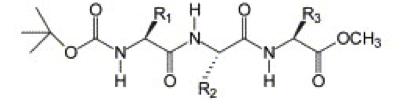
Figure 1 | Protected tripeptide from Ref. 5, R1 = R3 = TYR
2. Creating Peptide Coordinates
To simplify the tripeptide for this tutorial, we will treat Boc-Tyr-X-Tyr-OMe as a simple Tyr-X-Tyr peptide with uncharged termini, so that all parameters for coarse-graining are available within the Martini force field for proteins.[7] We want to test all 20 mutations of the middle amino acid (X). An easy way to create the 20 different peptide coordinates is using a molecular builder such as Avogadro in combination with the NAMD engine in VMD.
The files discussed here can be found in the directory 2_Creating_coordinates.
Go into the directory 2_Creating_coordinates to create 20 all-atom structures. Before you can proceed, you must edit the file make_peptides.sh to point to the executable of VMD on your system. Within the shell script, if necessary edit the line:
vmd='vmd'
Save the file, make sure make_peptides.sh is executable and execute the shell script to generate the 20 required pdb files.
> ./make_peptides.sh
If all is well, you have now generated 20 all-atom structures of tripeptides. You may check by opening one or more of the pdb-files in VMD.
If you are interested in the details of this procedure, read the text below. However, you may press on and get the simulation running first and then return to study the details. It's up to you!
The idea of generating coordinates for each peptides is to use a template structure for a tripeptide and use this template to graft TYR-X-TYR unto the side chains. To this end, generic tripeptide coordinates are provided in the file XYZ.pdb. If you inspect this file, you will see coordinates for an atomistic model containing only the backbone atoms. There are several ways to generate such a file. Avogadro was mentioned. Also pymol contains an amino-acid builder. Using pymol, the required template file can be generated as follows:
1. Start up pymol.
2. Find the menu Build, and from this menu select Residue->Glycine three times in a row. You should see the glycine tripeptide.
3. Find the menu File->Save Molecule , and save the coordinates just generated under the name XYZ.pdb.
4. Exit pymol.
5. Open the file XYZ.pdb in an editor. Delete all the lines defining a H-atom. Change the residue identifiers GLY to XXX, YYY, and ZZZ for the first, second, and third residues, respectively. No other changes are necessary. Save the file.
The script make_peptides.sh loops over all 20 amino acids and edits the template file XYZ.pdb and the script create_tripeptides.tcl to reflect the residues to be grafted unto the coordinate template to generate an instruction set for VMD. For each tripeptide, the script make_peptides.sh then calls VMD with this instruction set to generate the coordinates of the required tripeptide. The coordinates are based on the CHARMM all-atom force field, and the building blocks containing information to construct positions from back-bone coordinates only are contained in the file top_all36_prot.rtf. Note that the script make_peptides.sh can easily be modified to generate coordinates for all possible tripeptides.
3. Create a coarse-grained system using martinize.py and Gromacs tools
In this step, one or more of the atomistic structures generated in step 2, are used to generate a Martini coarse-grained topology file, a coarse-grained structure of a single tripeptide, and a simulation box containing 100 peptides and solvent randomly placed in the box. The files discussed here can be found in the directory 3_Coarse-graining.
Coarse-grained Martini topologies of peptides and proteins can be built automatically using the martinize.py script. An elaborate tutorial is available as part of the Protein tutorial on the Martini website.
Execute the martinize.py script on a tripeptide of your choice to create coarse-grained coordinates using the Martini 2.2 force field. Remember to use neutral termini! In the papers discussing the YXY peptide it is mentioned that the backbone dihedral angles in the crystal structure fall in the β-sheet Ramachandran region.[5,6] We therefore use the extended β secondary structure for all three amino acids (flag ‘–ss EEE’). In the commands below, replace XXX by the three-letter amino acid code of your choice:
> ./martinize.py –f ../2_Creating_coordinates/TYR-XXX-TYR_aa.pdb –name TYR-XXX-TYR –o TYR-XXX-TYR.top –x TYR-XXX-TYR.pdb –ff martini22 –nt –ss EEE
You need to edit the output file TYR-XXX-TYR.top. The martinize.py script adds an #include statement to the generic Martini force field file. Since we are using version 2.2, make sure the statement reads:
#include "martini_v2.2.itp"
Inspect the output file TYR-XXX-TYR.itp to see what bead types were chosen for different parts of the peptide. Does it make sense?
When you have the coarse-grained coordinates of a single peptide and created its topology, create a small box of water containing enough peptides to create a self-assembled structure. For this tutorial, a small box of 8 x 8 x 8 nm containing 100 peptides can be used. The Gromacs tool genbox enables you to first define the box and fill it with 100 peptides and next, fill the box containing the 100 peptides with Martini water. For more details, see the introductory lipid self-assembly tutorial.
> genbox –box 8 8 8 –nmol 100 –ci TYR-XXX-TYR.pdb –vdwd 0.4 –o TYR-XXX-TYR_box.gro
> genbox –cp YXY_box.gro –cs water-80A_eq.gro –vdwd 0.21 –o TYR-XXX-TYR_water.gro
N.B.1: the -vdwd flags keep the peptides somewhat apart initially (setting 0.4) and create a density that is roughly right for Martini water (setting 0.21). Note that the genbox tool contains a bug that adds too many water beads if you solvate with water boxes of significantly different sizes than the peptide box. If you plan to use a different sized simulation box, first create an equilibrated water box of that size. Here, the file water-80A_eq.gro contains Martini water in a container of the correct size.
N.B.2: You will have to edit the TYR-XXX-TYR.top file again to include the right number of peptides (100) and the right number of water beads (name W, check the output of the second genbox command for the amount).
N.B.3: Note that the concentration of peptides here is ~0.32 M. This is way higher than experimentally, but otherwise we might be waiting a long time for the peptides to assemble into a large enough aggregate! On the other hand, the nanostructures found were created by evaporation of solvent, and the local concentration of peptides close to the nanostructure may be a lot higher than the average concentration in the bulk anyway.
We have now generated a structure containing 100 peptides solvated in Martini water. Some peptides may be charged, however, and it is advisable to add at least counter ions. The Gromacs tool genion can replace water beads by ion beads based on the electrostatic potential at the water beads; it will replace the water bead by an ion bead where this is energetically most favorable. The new structure is written out and the topology file is adapted to reflect the change in number of water and ions. The tool genion requires a .tpr file. Generate this first and then replace water beads by ions:
> grompp -f tripep_water_min.mdp -p TYR-XXX-TYR.top -c TYR-XXX-TYR_water.gro -o TYR-XXX-TYR_genion.tpr
> genion -s TYR-XXX-TYR_genion.tpr -pname NA+ -nname CL- -neutral -o TYR-XXX-TYR_water.gro
N.B. 1 The names of the ions are added explicitly on the command line of genion to make sure they are compatible with the names of the ion beads in Martini (defined in the file martini_v2.0_ions.itp).
N.B. 2 The starting structure is given the same name as the one containing only water. This is done on purpose with automation in mind. If the system is neutral, no ions are added and no output is produced. If the name of the structure file would be different (e.g. TYR-XXX-TYR_wion.gro), scripts would have to check whether this file exists or whether the system was neutral.
Before leaving this section, if your peptide is not neutral and water beads were replaced by ion beads, edit the topology file for your peptide to reflect the fact that you have ion beads in the system by:
(i) adding an include statement (use a line below the main Martini include file) for the file defining Martini ion beads:
#include "martini_v2.0_ions.itp"
(ii) in the [molecules] section, change the number of water beads and add a line specifying the ion beads (the ions are all collected at the end of the structure file).
You may automatically perform this procedure for all 20 peptides by executing the script setup_tripeptides.sh.
4. Running self-assembly simulations
Now the starting structure(s) of 100 peptides in water in the Martini model are generated. The next step is to run the simulation(s) in which the peptides may or may not be seen to self assemble. The protocol is similar to that in lipid self assembly, see the introductory lipid self-assembly tutorial.
The files discussed here can be found in the directory 4_Running_simulations.
Standard minimization and equilibration MD inputs are provided. Inspect the files tripep_water_min.mdp and tripep_water_eq.mdp and rationalise the mdp options used. If you have time, perform the simulations for all the peptides, otherwise choose one peptide to take through the steps of this tutorial and use the output provided for the other peptides. 500,000 steps of 25 fs take about 7 minutes to complete on an 8-processor machine. In the commands below, replace XXX by the three-letter amino acid code of your choice:
> grompp -f tripep_water_min.mdp -p ../3_Coarse-graining/TYR-XXX-TYR.top -c ../3_Coarse-graining/TYR-XXX-TYR_water.gro -o TYR-XXX-TYR_min.tpr
> mdrun -deffnm TYR-XXX-TYR_min -v
> grompp -f tripep_water_eq.mdp -p ../3_Coarse-graining/TYR-XXX-TYR.top -c TYR-XXX-TYR_min.gro -o TYR-XXX-TYR_eq.tpr -maxwarn 1
> mdrun -deffnm TYR-XXX-TYR_eq -v
All tripeptides can sequentially be treated in this manner automatically by running the script run_sims.sh. This may take prohibitively long, and if you want to test the automated analysis in the next step, it is best done by continuing in the directory 4_Done that contains all simulations.
5. Analysing the results
The files discussed here can be found in the directory 5_Analysis. In the commands below, replace XXX by the three-letter amino acid code of your choice.
Inspect the results of the simulation using VMD.
> vmd ../4_Running_simulations/TYR-XXX-TYR_min.gro ../4_Running_simulations/TYR-XXX-TYR_eq.xtc
Since we are looking at a coarse-grained model, VMD does not show a bond structure on the peptides. You must change the representation of the particles to get a better view. The simplest action is to open the Graphics->Graphical Representations menu, in the Selected Atoms window type not name W, and in the Drawing Method window select VDW. This will show the peptides in a rough-and-ready form. It is not the best representation, however, and you may need a better view. Please consult the tutorial on visualization Martini using VMD.
Do you find any nanotubes? Can you explain why (not)?
You may or may not be lucky and have a single aggregate that is not split across the periodic boundary. The clusters of peptides are often spread across the periodic boundaries of the system for most systems. You can centre the final snapshot on a large cluster using:
> echo 1 1 1 | trjconv –f ../4_Running_simulations/TYR-XXX-TYR_eq.gro –s ../4_Running_simulations/TYR-XXX-TYR_eq.tpr –pbc cluster –center –o TYR-XXX-TYR_clustered.gro
Now, open the clustered final snapshot in VMD and adapt the representation (note, is no solvent in the file anymore).
As you will notice when you compare different tripeptides, the tyrosine residues strongly drive aggregation in water, irrespective of the middle amino acid. However, you should be able to distinguish slightly different levels of aggregation for different peptides. One way to quantify the level of aggregation is calculating the solvent-accessible surface area (SASA) after assembly and compare to the initial SASA after energy minimization of the box.[4,8] Take the ratio SASAinitial / SASAfinal as a measure for the aggregation propensity using the Gromacs command g_sas.
> echo 1 1 | g_sas –f ../4_Running_simulations/TYR-XXX-TYR_min.gro –s ../4_Running_simulations/TYR-XXX-TYR_min.tpr –o TYR-XXX-TYR_sasa_init.xvg
> echo 1 1 | g_sas –f TYR-XXX-TYR_clustered.gro –s ../4_Running_simulations/TYR-XXX-TYR_eq.tpr –o TYR-XXX-TYR_sasa_end.xvg
N.B. If you have time or are interested: you can also calculate the SASA for an assembly using the VMD tool measure, where a rolling sphere (e.g. of radius 1.4 nm) is used to determine the SASA of a selection of atoms. Does it match the result from g_sas? Start up VMD (in the directory 4_Running_simulations) and in the Tk console of VMD, type:
mol new TYR-XXX-TYR_min.gro
set sasa_ini [measure sasa 1.4 [atomselect top “not resname W and not resname ION”]]
mol new ../5_Analysis/TYR-XXX-TYR_clustered.gro
set sasa_end [measure sasa 1.4 [atomselect top “not resname W and not resname ION”]]
set aggregation_propensity [expr $sasa_ini / $sasa_end]
echo $aggregation_propensity
The change in solvent accessible surface is a measure of the level of aggregation. However, the level of aggregation is not a direct measure for the suitability of a peptide to create a well-ordered nanostructure under aqueous conditions, as it can also mean the peptide is not actually soluble, or simply forms disordered aggregates. To get more insight into the structure and organization within the assembly, you can for example try to calculate molecular order through radial distribution functions. Another example is looking for 1-dimensionality as is typically observed in self-assembled peptides that form fibres or tubes. A basic indication of the shape can be automated using Gromacs’s built-in tools as outlined below. For more advanced ways to calculate a nanostructure’s shape, see ref.[9].
We will calculate the moments of inertia (MOIs) along the principal axes of the system of the largest cluster of peptides only. Note that it requires the creating of some extra .tpr files to persuade Gromacs to work on the right molecules in the cluster. First, we make an index file containing the peptides only:
> make_ndx –f ../4_Running_simulations/TYR-XXX-TYR_eq.gro –o TYR-XXX-TYR_noW.ndx < options.txt
Next, the Gromacs tool g_clustsize is used to extract the largest cluster from the final snapshot, based on a distance criterion of 0.5 nm. The indices (bead numbers) of the beads involved in the largest cluster are written to the index file TYR-XXX-TYR_maxclust.ndx.
> g_clustsize –f ../4_Running_simulations/TYR-XXX-TYR_eq.gro –s ../4_Running_simulations/TYR-XXX-TYR_eq.tpr –mcn TYR-XXX-TYR_maxclust.ndx –n TYR-XXX-TYR_noW.ndx –cut 0.5
The next step is to create a new .tpr file for the selected atoms and to use this .tpr file to center the cluster and to align it according to its principal axes for visualization; the snapshot TYR-XXX-TYR_princ.gro generated using the Gromacs command editconf contains the aligned cluster. Comparing these snapshots from different tripeptides should give some insight into the differences in self-assembled structures.
> tpbconv –s ../4_Running_simulations/TYR-XXX-TYR_eq.tpr –n TYR-XXX-TYR_noW.ndx –nsteps -1 –o TYR-XXX-TYR_noW.tpr
> trjconv –f TYR-XXX-TYR_clustered.gro –s TYR-XXX-TYR_noW.tpr –n TYR-XXX-TYR_noW.ndx –o TYR-XXX-TYR_maxclust.gro
> tpbconv –s TYR-XXX-TYR_noW.tpr –n TYR-XXX-TYR_maxclust.ndx –nsteps -1 –o TYR-XXX-TYR_maxclust.tpr
> echo 1 | editconf –f TYR-XXX-TYR_maxclust.gro –princ –c –o TYR-XXX-TYR_princ.gro
Finally, the Gromacs tool g_gyrate is used to calculate the MOIs.
> echo 1 | g_gyrate –f TYR-XXX-TYR_princ.gro –s TYR-XXX-TYR_maxclust.tpr –moi –o TYR-XXX-TYR_gyrate.xvg
The moments of inertia of the cluster in the final snapshot is written to the .xvg file, which is human readable. Calculate the aspect ratios (Iz / Ix). Aggregates with Ix << Iy ≈ Iz are mainly 1D.
If you have done all peptide self assembly simulations, or want to look at the provided final structures of all 20 peptides, start up VMD and type source load_tripeptides.tcl into the VMD Tk console to load all peptides at once into VMD.
You can perform the analysis for all peptides in automated fashion using the analysis.sh script. Summaries of the analysis are written to the files sasa_trip.txt and inertia_trip.txt. Which peptides are the most fibrous?
Tools and scripts used in this tutorial
gromacs (http://www.gromacs.org/)
insane.py (downloadable here)
[1] Reches, M., and Gazit, E. Casting metal nanowires within discrete self-assembled peptide nanotubes. Science 300, 625–627 (2003).
[2] Ghadiri, M. R., Granja, J. R., Milligan, R. A., McRee, D. E., and Khazanovich, N. Self-assembling organic nanotubes based on a cyclic peptide architecture. Nature 366, 324–327 (1993).
[3] Zhang, S., Holmes, T., Lockshin, C. & Rich, A. Spontaneous assembly of a self-complementary oligopeptide to form a stable macroscopic membrane. Proc. Natl. Acad. Sci. U. S. A. 90, 3334 –3338 (1993).
[4] Frederix, P. W. J. M. et al. Exploring the sequence space for (tri-)peptide self-assembly to design and discover new hydrogels. Nat. Chem. 7, 30–37 (2015).
[5] Ray, S., Haldar, D., Drew, M. G. B. & Banerjee, A. A New Motif in the Formation of Peptide Nanotubes: The Crystallographic Signature. Org. Lett. 6, 4463–4465 (2004).
[6] Ray, S., Drew, M. G. B., Das, A. K. & Banerjee, A. The role of terminal tyrosine residues in the formation of tripeptide nanotubes: a crystallographic insight. Tetrahedron 62, 7274–7283 (2006).
[7] Monticelli, L. et al. The MARTINI Coarse-Grained Force Field: Extension to Proteins. J. Chem. Theory Comput. 4, 819–834 (2008).
[8] Frederix, P. W. J. M., Ulijn, R. V., Hunt, N. T. & Tuttle, T. Virtual Screening for Dipeptide Aggregation: Toward Predictive Tools for Peptide Self-Assembly. J. Phys. Chem. Lett. 2, 2380–2384 (2011).
[9] Fuhrmans, M. & Marrink, S.-J. A tool for the morphological analysis of mixtures of lipids and water in computer simulations. J. Mol. Model. 17, 1755–1766 (2011).
Hybrid model using virtual sites
- Details
-
Last Updated: Wednesday, 26 August 2015 05:33
Martini tutorials: hybrid model using virtual sites
Summary
Aim
Background
1. The Models
2. The Combination of the Models
3. Setting up and Running the Hybrid System
4. Fine-graining a Hybrid Snapshot
5. Setting up a System involving Charged Peptides and Ions
Appendices
Aim
Demonstrate how to combine different Classical Mechanical level models within GROMACS and run a HYBRID simulation. In general, this will involve providing user-defined tabulated potentials to GROMACS. A second aim is to demonstrate a back-mapping procedure to build (partially) atomistic structures from (fully/partially) coarse-grained models.
Background
Many properties of molecular systems are local, i.e. primarily determined by the molecule and its nearest neighbors. Simulations of small systems therefore often already provide a reasonable to good representation of macroscopic systems. Nevertheless, small system simulations may contain artifacts due to the boundary conditions placed on them. Also, the minimal size of the simulated systems may still prevent sufficient sampling of phase space. The idea of HYBRID models is that a detailed description of relatively distant molecules is not required and that enhanced sampling of a region of interest may be achieved by embedding it in a surroundings that represents the environmental influences properly but at a computationally less demanding level. This approach has long been applied to the combination of quantum chemistry and molecular mechanics models (QM/MM), but is much less well developed for combining molecular models at different levels of resolution. It should be kept in mind that developments in this area are still ongoing and that there is as of yet no standard or best practice for this type of simulations.
In this tutorial, we shall focus on the combination of an atomistic (AA, or fine-grained, FG) and a coarse-grained (CG) model. The coarse-grained model is one employing a particle — as opposed to a continuum — description of the surroundings. The standard machinery present in GROMACS allows a quite generic implementation of HYBRID particle-based models through using VIRTUAL sites for the particles at the coarser level in addition to the normal atoms at finer level, and possibly adding user-defined interactions between the particles in accordance with the appropriate expression for the total energy.
The correspondence between the atoms and the virtual sites is called the MAPPING of the atomistic to the CG model. A CG model by itself may use such mapping schemes to parameterize (parts of) the force field. In a purely hierarchical scheme, such as force matching, atomistic simulations are used to calculate the forces on the mapped centers, which are then averaged over many snapshots to define the interactions between the CG particles. In an empirical approach, such as the Martini model, the bonded interactions between CG particles are often refined based on atomistic simulations; the distributions of bond lengths, bond angles and torsional degrees of freedom at the CG level are compared to those from the mapped atomistic simulations and bonded parameters are adapted to get an overall reasonable agreement. Tutorials involving fine-tuning can be found here and in the lipid and polymer tutorials. The non-bonded interactions in the Martini model are nevertheless generic and based on parameterization to experimental data.
Hybrid OPLS-AA/L—Martini model
The material presented in this tutorial leans on the work originating in the Molecular Dynamics Group at the University of Groningen, in particular that by Tsjerk Wassenaar. The two main publications primarily concern the combination of GROMOS united atom and Martini force fields. Here, we show that one can combine OPLS-AA/L and Martini in the same fashion.
GROMACS implements a considerable number of standard interaction potentials, both bonded and non-bonded. It also enables the users to define their own interaction potentials. In addition, the code implements the generation and use of interaction centers (called VIRTUAL sites) whose positions depend in some geometrically well-defined way on the positions of two or more other particles. A hybrid model combines molecular models at different levels of resolution. The different models may use different types of interaction potentials, and may therefore not be compatible with the same non-bonded (and bonded) functional forms, necessitating a more complex set-up of hybrid model simulations than simulations at a single level of resolution. Here, a set-up will be demonstrated for a combination of the OPLS-AA/L peptide model with the Martini coarse-grained model. The peptide will interact internally at the atomistic resolution, while it interacts with solvent at the coarse-grained (CG) level. The solvent interacts with itself only at CG level. Sections 1-3 take you through setting up and running such a hybrid system for a single AA peptide in Martini water.
In Section 4 a tool is introduced to generate fully atomistic solvent configurations from the hybrid simulation that can serve as starting points for production runs at all-atom (AA) level. Such procedures are known as back-mapping techniques.
Section 5 uses the back-mapping tool to generate coordinates for a hybrid simulation from a fully coarse-grained snapshot. Here, a collection of peptides is back-mapped from the Martini model to the OPLS-AA/L model, while the water and coarse-grained ions are maintained at the Martini level.
All files are provided in the tar-ball hybrid-tutorial.tgz, which expands to the main directory hybrid-tutorial/OPLS-MARTINI. Paths will be given with respect to this directory. A directory with all the results is provided in the tar-ball hybrid-tutorial-worked.tgz, under hybrid-tutorial/WORKED.
1. The Models
A. Atomistic model: OPLS-AA/L
As atomistic model we will use the OPLS-AA/L force field.[1] Here, we will have a peptide interacting internally through this force field. The standard atomistic model can be built using the GROMACS tool pdb2gmx. Here, we will use a small tripeptide, TYR-VAL-TYR, with methylated terminal ends. A Protein Data Bank (PDB) file can be built very simply using e.g. the builder of pymol, or by finding an existing protein in the PDB with this sequence of residues and cutting those out. We wish to use neutral methylated end-groups, normally known in the PDB as ACE for the C-terminal end and NMA for the N-terminal end. To make this work with the standard library file for OPLS-AA/L in GROMACS, the residue name of the N-terminal end must be changed manually from NMA to NAC.
Hands-on
Go to the directory OPLSAA. The file YVY.pdb (Tyr-Val-Tyr), built using pymol, is available for you, and it incorporates the naming of the N-terminal end (NAC instead of NME, done by manual editing) to comply with the GROMACS implementation of the OPLS-AA/L force field. Build the atomistic topology file:
> pdb2gmx -f YVY.pdb -ter -ignh
This command generates an OPLS-AA peptide topology, topol.top, after ENTERING the correct numbers (which may depend on the exact GROMACS version) for the options OPLS-AA/L force field, TIP3P for the water model, and None for both terminal ends.
B. Coarse-grained solvent model: Martini
As a solvent, the Martini model for water and hydrated ions will be used.[2] This model will also deal with the interactions between the peptide and the solvent and hydrated ions (see Section 2 for further details). Standard Martini files can be downloaded (but that is not necessary here because they are provided for you) from the Martini website. They cannot be used as such, however, in the hybrid set-up, and modifications will need to be made. The standard file for the Martini model which serves as the basis for the modifications can be found in the directory SOLVENT/martini_v2.2.itp.
2. The Combination of the Models
Models at different levels can be combined in a number of schemes. We describe the simplest approach, viz. we choose to administer all interactions as being at either AA or CG level. The particles making up the peptide will interact at both atomistic and coarse-grained levels. Within the peptide, the interactions should be treated according to the atomistic force field. The atoms of the peptide see the other atoms of the peptide as they would in a normal atomistic simulation. Interactions of the peptide with the solvent are to be CG interactions, i.e. treated entirely according to the Martini model. This clear-cut separation is possible for the system defined here because there are no Coulomb interactions between the AA and CG subsystems. Standard Martini water beads are single, neutral particles. (The proper treatment of electrostatic interactions across the two levels is by no means a finished area of research. Aspects are discussed in Section 5.)
The present set-up achieves the separation between AA and CG interactions by adding VIRTUAL sites to the atomistic topology, and making sure that these sites have no interaction with the atoms, nor with each other, but only with the solvent. The atomistic topology generated for the peptide must be extended with the virtual sites to build a hybrid topology for the peptide.
A. HYBRID TOPOLOGY FOR THE PEPTIDE
The hybrid topology for the peptide makes use of VIRTUAL SITES. These are described in the GROMACS manual in Section 4.7. In the present implementation, the virtual sites are defined as the centers of mass of a number of atoms. The virtual sites themselves are also particles belonging to the molecule. Thus, two entries need to be ADDED to the atomistic topology. The first extension is either an extension of the [ atoms ] directive containing the atomistic particles or a second [ atoms ] directive placed somewhere below the first one. In both cases, the atom numbering must be consecutive to the atoms already defined. The second extension is a [ virtual_sitesn ] directive, which defines how the added virtual sites are related to the normal atoms of the molecule. The additional virtual sites and the mapping can be added by hand, but a script is also available to do this for you. The conf.gro file of the peptide generated by pdb2gmx can be used to generate a Martini topology using an adapted martinize.py script (available in HYBRIDTOPOLOGY — the original script is downloadable from the Martini web-site) after slight modification of the terminal methylated groups. The standard Martini model does not implement the neutral methylated terminal ends. To distinguish them properly in the martinize.py script, a name change of the methyl carbon is required.
Hands-on
Go to the directory HYBRIDTOPOLOGY. Copy the standard pdb2gmx output file conf.gro produced in Section 1 to conf-martini.gro and edit the CH3 of the ACE residue to be named CTJ and the CH3 of the NAC residue to be named CTB. This change is for the benefit of making the adapted martinize-ter.py script recognize these neutral methylated termini.
> cp ../OPLSAA/conf.gro ./conf-martini.gro
> [vi/gedit] conf-martini.gro
Edit the conf-martini.gro to look like this:
Gallium Rubidium Oxygen Manganese Argon Carbon Silicon
70
1ACE CTJ 1 -1.244 0.089 -0.561
1ACE HH31 2 -1.272 0.187 -0.524
1ACE HH32 3 -1.199 0.101 -0.659
1ACE HH33 4 -1.333 0.029 -0.571
1ACE C 5 -1.146 0.024 -0.467
1ACE O 6 -1.176 0.001 -0.349
...
5NAC N 55 -0.107 -0.003 0.013
5NAC H 56 -0.153 0.028 0.100
5NAC CTB 57 0.034 0.012 -0.021
5NAC HH31 58 0.062 -0.063 -0.094
5NAC HH32 59 0.052 0.110 -0.062
5NAC HH33 60 0.094 -0.001 0.068
1.42700 0.79900 0.81020
Now, execute the martinize-ter.py script (this is the adapted version):
> python martinize-ter.py -f conf-martini.gro -ff martini22 -multi all -nt -o martini.top -x hybrid.pdb
This generates an extension to the molecule definition of the tri-peptide, defining 12 new atom entries that are defined as virtual sites. The flag -ff selects the Martini force field version, the flag -multi all produces a topology extension for hybrid AA-CG simulations (omitting this flag, you get a topology for pure Martini CG simulations), the flag -nt ensures neutral termini, and the -x flag produces a starting structure including the virtual sites. The topology extension is written to the standard file Protein_A.itp, which should look like the text shown below:
; MARTINI (martini22) Multiscale virtual sites topology section for "Protein_A"
; Sequence:
; JYVYB
; Secondary Structure:
; CCCCC
[ atoms ]
71 vN0 1 ACE vBB 71 0.0000 ; C
72 vP5 2 TYR vBB 72 0.0000 ; C
73 vSC4 2 TYR vSC1 73 0.0000 ; C
74 vSC4 2 TYR vSC2 74 0.0000 ; C
75 vSP1 2 TYR vSC3 75 0.0000 ; C
76 vP5 3 VAL vBB 76 0.0000 ; C
77 vAC2 3 VAL vSC1 77 0.0000 ; C
78 vP5 4 TYR vBB 78 0.0000 ; C
79 vSC4 4 TYR vSC1 79 0.0000 ; C
80 vSC4 4 TYR vSC2 80 0.0000 ; C
81 vSP1 4 TYR vSC3 81 0.0000 ; C
82 vN0 5 NAC vBB 82 0.0000 ; C
;
; Coarse grained to atomistic mapping
;
#define mapping virtual_sitesn
[ mapping ]
71 2 1 2 3 4 5 6
72 2 7 8 9 10 26 27
73 2 11 14 15 16
74 2 17 18 21 22
75 2 19 20 23 24 25
76 2 28 29 30 31 42 43
77 2 32 33 34 35 36 37 38 39 40 41
78 2 44 45 46 47 63 64
79 2 48 51 52 53
80 2 54 55 58 59
81 2 56 57 60 61 62
82 2 65 66 67 68 69 70
Each virtual site is defined as the center of mass of a number of atoms of the tri-peptide. The virtual sites are given first, under the [ atoms ] directive, and are numbered starting from 71; the all-atom model tri-peptide has 70 atoms. The atom types given to the virtual sites are those of the Martini model for proteins and peptides, with a prefix v (e.g., the standard back-bone bead for a coil residue in Martini is P5; therefore the bead-type for the back-bone beads 72, 76, and 78 are vP5). The mapping is defined in the directive [ mapping ], which is made to be interpreted by grompp as a directive [ virtual_sitesn ]. The first number is the index number of the virtual site, the second number (2 for all sites) specifies the type of virtual site (center of mass), and the other numbers are the indices of the atoms that define the virtual site. You may cross-check the mapping with the atom definition given in the atomistic topology.
To weave the two models together, copy the topol.top obtained from the atomistic model to hybrid.top.
> cp ../OPLSAA/topol.top ./hybrid.top
> [vi/gedit] hybrid.top
Use an editor to add the Martini addition in Protein_A.itp at the appropriate place, which is just after the definition of the peptide ends. Excerpts of the file hybrid.top are shown below:
; Command line was:
; pdb2gmx -f YVY.pdb -ter -ignh
;
; Force field was read from the standard Gromacs share directory.
;
; Include forcefield parameters
#include "oplsaa.ff/forcefield.itp"
[ moleculetype ]
; Name nrexcl
Protein 3
[ atoms ]
; nr type resnr residue atom cgnr charge mass typeB chargeB massB
; residue 20 ACE rtp ACE q 0.0
1 opls_135 1 ACE CH3 1 -0.18 12.011 ; qtot -0.18
2 opls_140 1 ACE HH31 1 0.06 1.008 ; qtot -0.12
...
69 opls_140 5 NAC HH32 25 0.06 1.008 ; qtot -0.06
70 opls_140 5 NAC HH33 25 0.06 1.008 ; qtot 0
[ bonds ]
...
[ pairs ]
...
[ angles ]
...
69 67 70 1
[ dihedrals ]
...
...
63 67 65 66 1 improper_Z_N_X_Y
; MARTINI (martini22) Multiscale virtual sites topology section for "Protein_A"
; Sequence:
; JVVVB
; Secondary Structure:
; CCCCC
[ atoms ]
71 vN0 1 ACE vBB 71 0.0000 ; C
...
82 vN0 5 NAC vBB 82 0.0000 ; C
;
; Coarse grained to atomistic mapping
;
#define mapping virtual_sitesn
[ mapping ]
71 2 1 2 3 4 5 6
...
82 2 65 66 67 68 69 70
; Include Position restraint file
...
[ system ]
; Name
Protein
[ molecules ]
; Compound #mols
Protein 1
B. HYBRID FORCE FIELD FILES
We now have a topology for the hybrid peptide model. In general, further modifications are required before we can run a simulation. First of all, the virtual sites constitute atom-types belonging to the CG model that are not known in the atomistic force field. They must be added to the atom-type list. Of course, the atom-type definitions must not overlap between the two models. For the combination of OPLS-AA/L and Martini this is no problem, but in general, you may need to rename the atom-types of either force field. Also, interactions must be defined between the sets of the two different force fields: either they must be set to zero, or defined explicitly if required. In GROMACS, standard files for interactions are provided for a number of force fields in libraries, provided in directories, see the GROMACS manual, Section 5.8. The OPLS-AA/L force field definitions can be found in the directory YOUR-PATH-TO-GROMACS/share/gromacs/top/oplsaa.ff. We will need to adapt the file ffnonbonded.itp in this directory. Since we may not have administrative privileges, we will copy the entire directory to a place that is under our control, effect the required changes there and make sure those files are used in our simulations.
Hands-on
Go to the directory FORCEFIELDS, and copy the standard library directory (or use the one already copied for you there):
> cp -R YOUR-PATH-TO-GROMACS/share/gromacs/top/oplsaa.ff .
> cd oplsaa.ff
Valid atom-types for any force field are defined in the file ffnonbonded.itp under the directive [ atomtypes ]. In the GROMACS implementation of the OPLS-AA/L force field there is a long list of atom types. For each atom type, the Lennard-Jones sigma and epsilon values are given in the 7th and 8th column of each entry. An excerpt of the file ffnonbonded.itp is given below to illustrate the point.
[ atomtypes ]
; full atom descriptions are available in ffoplsaa.atp
; name bond_type mass charge ptype sigma epsilon
opls_001 C 6 12.01100 0.500 A 3.75000e-01 4.39320e-01 ; SIG
opls_002 O 8 15.99940 -0.500 A 2.96000e-01 8.78640e-01 ; SIG
...
The nonbonded interaction parameters can be calculated from the values entered using standard combination rules. GROMACS implements and geometric and arithmetic means, specified in GROMACS in the [ defaults ] directive, which can be found in the forcefield.itp file. In addition, the interaction parameters for pairs of types can be set explicitly, overriding the standard values. This is done in the [ nonbond_params ] directive in the file ffnonbonded.itp. Since OPLS-AA/L uses standard combination rules, the [ nonbond_params ] directive is missing from the file ffnonbonded.itp. You may skip the OPTIONAL part below if you like and continue at the end of the OPTIONAL part.
OPTIONAL (intermediate step)
Just adding the Martini types used for the virtual sites as valid OPLS-AA atom types (make sure you define them as type V, not A) with standard LJ parameters 0 and 0, allows you to do a simulation in vacuum with the virtual sites present, but not interacting with anything. You may attempt to add the virtual site types yourself by hand (you will need vN0, vP5, vSC4, vSP1, and vAC2), or copy the pre-prepared force field files in which this edit has been done for you.
Hands-on
Go to the VACUUM directory and either copy the given files:
> cp -R ../FORCEFIELDS/hyb-vac.ff oplsaa.ff
or copy the standard files and edit the file ffnonbonded.itp:
> cp -R gromacs_path/share/gromacs/top/oplsaa.ff .
> [vi/gedit] oplsaa.ff/ffnonbonded.itp
Next, copy your hybrid starting structure and edited topology there, and you should be able to run a vacuum simulation using the provided set-up file sd.mdp (using straight cut-off Coulomb interactions instead of PME and without pressure correction):
> cp ../HYBRIDTOPOLOGY/hybrid.pdb .
> cp ../HYBRIDTOPOLOGY/hybrid.top .
> grompp -p hybrid.top -c hybrid.pdb -f sd.mdp -maxwarn 1
> mdrun -v
> vmd -e viz-sdrun.vmd
When visualizing with vmd, using the .vmd file, you will see the virtual sites, the positions of the Martini beads as green spheres. Due to the standard settings of vmd drawing bonds on the basis of distances, bonds will be drawn between the virtual sites and nearby atoms.
END OPTIONAL
The MARTINI force field has interaction levels that do not follow from a multiplication rule; it therefore defines a full matrix of interactions. The interaction matrix between Martini beads must be added to the nonbonded definition file in the [ nonbond_params ] directive of the file ffnonbonded.itp. Interactions must be defined between the sets of the two different force fields: either they must be set to zero, or defined explicitly if required. This can be done by hand by appropriately mixing the two files and extending the table with pairs of interactions. Finally, in general one may not want all molecules of a particular kind to interact at a particular level, but only a limited sub-set. For example, we may want to study the active site of a protein atomistically, but embedded in a CG protein and CG water. The virtual sites representing the CG active site must not interact with each other (the atomistic interactions take care of that), but should interact with all surrounding molecules in the appropriate CG manner. One could generate a list of exclusions for the virtual sites while using their normal CG atom types. A more general approach is to double the type of interactions, here CG, where a distinction is made between the types that do not interact with each other, here with prepended v, e.g. vP5 for a P5-type particle, and the normal CG types. Now v-particles can interact with all CG particles in the normal CG manner, whereas they do not interact at all amongst themselves if the LJ parameters between all v-particles are set to zero. This approach is followed here, and you may try to edit an appropriate file yourself, or use a minimal nonbonded file defined for you in FORCEFIELDS/hybrid.ff/ffnonbonded.itp.
You may skip the OPTIONAL part below if you like and use the pre-prepared force field files in which this edit has been done for you (FORCEFIELDS/hybrid.ff/ffnonbonded.itp) and continue at the end of the OPTIONAL part.
OPTIONAL (defining the set of CG and virtual particle interactions)
Hands-on
Go to the FORCEFIELDS directory and make a copy of the OPLS/AA force field files:
> cp -R oplsaa.ff myhybrid.ff
Open the file myhybrid.ff/ffnonbonded.itp and add the Martini types used for the coarse-grained system and for the virtual sites as valid OPLS-AA atom types (make sure you define the ones for the virtual sites as type V, not A) with standard LJ parameters 0 and 0 (you will need P4, BP4, vN0, vP5, vSC4, vSP1, and vAC2).
> [gedit/vi] myhybrid.ff
Next, while still in the editor, add a directive [ nonbond_params ] and specify explicitly the non-bonded interaction matrix for interactions that should be non-zero. If a pair is not specified in the [ nonbond_params ] directive, standard combination rules will be used; thus by defining a particle type with LJ parameters 0 and 0 this type will always have no LJ interaction with any other particle type if the pair interaction is not explicitly defined in the [ nonbond_params ] directive. An example of a [ nonbond_params ] directive entry is shown below.
[ nonbond_params ]
; type1 type2 flag sigma epsilon
P5 P5 1 0.47e-00 0.56e+01 ; supra atrractive Martini interaction
When you are done, you may compare your file myhybrid.ff/ffnonbonded.itp with the file hybrid.ff/ffnonbonded.itp.
END OPTIONAL
NOTE that the standard Martini force field file available from the Martini website (and provided in the SOLVENT directory) uses C6 and C12 parameters instead of sigma and epsilon, as appropriate for the OPLS-AA/L force field. Thus, the Martini parameters must now also be specified in terms of sigma and epsilon (which is the way they are defined in Martini papers).
3. SETTING UP AND RUNNING THE HYBRID SYSTEM
We will now work toward a hybrid simulation of a single atomistic tripeptide solvated in Martini water.
A. Surrounding the solute with solvent
First, a starting structure must be prepared in which the peptide is solvated. GROMACS has a standard tool to solvate systems, genbox. One can either use an equilibrated solvent box to fill an existing system containing a solute, or insert individual molecules one by one. After one or more molecules are inserted, a check for close contacts is made and new molecules that are too close to existing molecules are removed.
Hands-on
Go to the HYBRID directory. Take the hybrid solute co-ordinates, center them in the box and define a box-size of 3.5x3.5x3.5 nm, and fill this with Martini water beads. A co-ordinate file containing 400 equilibrated Martini waters (water.gro) is available from the Martini web-site, and is also provided for you in the SOLVENT directory.
> cp ../SOLVENT/water.gro .
> editconf -f ../HYBRIDTOPOLOGY/hybrid.pdb -center 1 1 1 -box 3.5 3.5 3.5
> genbox -cp out.gro -cs water.gro -o solvated.gro -vdwd 0.2
> cp ../HYBRIDTOPOLOGY/hybrid.top .
Edit the topology file (hybrid.top) to include the definition of the Martini water bead (define a moleculetype or use a #include; the file SOLVENT/MartiniWater.itp contains it) and specify the number of water beads just added to your system (right at the bottom in the [ molecules ] directive; the Martini water bead is called W). The number of water beads added should be clear from the output of the genbox command.
> [vi/gedit] hybrid.top
Next, either copy the directory with pre-edited OPLS-AA/L force field files:
> cp -R ../FORCEFIELDS/hybrid.ff oplsaa.ff
or copy the directory with the standard OPLS-AA/L force field files and edit them to include the Martini-bead definitions (see the OPTIONAL hands-on section just prior to this section):
> cp -R gromacs_path/share/gromacs/top/oplsaa.ff .
> [vi/gedit] oplsaa.ff/ffnonbonded.itp
OPTIONAL (intermediate stage)
The system thus defined will run; you can test this (in an energy minimization run) by running:
> grompp -p hybrid.top -c solvated.gro -f em.mdp -o em -maxwarn 1
> mdrun -v -deffnm em
> vmd -e viz-em.vmd
END OPTIONAL
B. Generating proper tabulated potentials
Just by making all CG atom types known to the OPLS-AA/L force field and adding the LJ-parameters, the simulation will run, but it is not a proper hybrid simulation because the two force fields do not use the same cut-offs for the nonbonded interactions, nor — in the case of OPLS-AA/L and Martini — the same functional form for the Coulomb and LJ interactions. If you would run an MD simulation with the present set-up, the density of the system is incorrect because with standard LJ potentials you would not get the proper density of Martini water.
The next ingredient is thus making sure that the interactions are treated properly according to the appropriate force fields. This may or may not be entirely possible within GROMACS. A powerful tool that enables multiscale simulations are the so-called “tables” that GROMACS implements. Internally, potentials and forces are tabulated within GROMACS and the forces are determined by an interpolation scheme between the tabulated values. This is hidden from the user, but users may define their own interaction tables, by which they can input any pairwise nonbonded interaction potential. The next section briefly takes you through the setting up of such tables. They are described in the GROMACS manual, Section 6.9 and a more extensive tutorial is available from the GROMACS website.
Nonbonded interaction tables can be defined for the interactions between any number of groups. Here, we need the following set, which are provided for you in the FORCEFIELDS directory:
(i) interaction tables between the atomistic particles, which will be called AA:
— the OPLS-AA/L force field with nonbonded cut-off of 1.0 nm, using a standard LJ potential contained in the file tables_AA_AA.xvg,
(ii) interaction tables between coarse-grained particles, which will be called CG:
— the MARTINI force field with nonbonded cut-off of 1.2 nm, using a modified LJ potential, contained in the file tables_CG_CG.xvg, and
(iii) interaction tables between the two types (AA and CG) of particles:
— for the example here, the potentials can be set to zero for all distances, but a file with these values must be present. We use the naming convention of GROMACS and let this interaction be the default, which means these interactions must be contained in the file table.xvg.
Each tables file contains 7 columns, the first column contains the distances between the pair of particles (in nanometer), and the next six columns implement three generic functions in three pairs of potential and force. Within GROMACS, the magnitude of the interaction or force is determined by the interpolated value taken from the tables file, multiplied by the appropriate Coulomb or LJ prefactors for the pair at hand. The structure of the tables files is thus:
distance f(r) f’(r) g(r) g’(r) h(r) h’(r)
and with heavily truncated numbers could start like this:
0.0000E+00 0.0000E+00 0.0000E+00 0.0000E+00 0.0000E+00 0.0000E+00 0.0000E+00
0.2000E-02 0.4999E+03 0.2499E+06 -0.1562E+17 -0.4687E+20 -0.2441E+33 0.1464E+37
....
For the first interaction (modeled on the Coulomb interaction), the prefactor for the functions f(r) and f’(r) is calculated by multiplication of the two charges and dividing by the dielectric constant (epsilon_r in the mdp-file). For the second (g) and third (h) functions, (modeled on the LJ interaction), the prefactors are calculated from the standard combination rules for the C6 and C12 parameters, respectively (which may themselves be calculated from the input sigma and epsilon values), or taken directly from the [ nonbonded_params ] list in the ffnonbonded.itp file. The distance spacing of the table files can be chosen at will but needs to be uniform. The tables should extend to at least the longest cut-off used in the interactions between the different types of particles, here 1.2 nm, but it is useful to make them extend beyond this — by default, tables are extended 1 nm beyond the cut-off (mdp option table-extension).
GROMACS provides a number of tables files for you, for example for the Lennard-Jones 6-9 potential, table6-9.xvg. They are provided in the YOUR-PATH-TO-GROMACS/share/gromacs/top directory, with an extension up to 3.0 nm. You will generally need to generate these files yourself, writing a script, a program, etc. Force-matching or related hierarchical coarse-grained force fields[3] generally use tabulated potentials derived from atomistic simulations. For the purpose of this tutorial, the tables files are provided for you in the FORCEFIELDS directory and you can simply copy them over. Technical information about the functional forms of the potentials used here is given in the appendix to a paper by Baron et al.[4]. NOTE that you also need a separate tablep.xvg file for 1-4 (pair) interactions.
OPTIONAL Hands-on
Go to the FORCEFIELDS directory. The tabulated potentials can be viewed using xmgrace, for example:
> xmgrace -nxy table_CG_CG.xvg -p xmgr.par
Return to the HYBRID directory.
END OPTIONAL
A basic mdp-file for energy minimization in the hybrid scheme using user-defined potentials is shown below (and provided for you as min.mdp):
; RUN CONTROL PARAMETERS
integrator = steep
nsteps = 100
; OUTPUT CONTROL OPTIONS
; Output frequency for coords (x), velocities (v) and forces (f)
nstxout = 1
nstvout = 1
nstenergy = 1
; Selection of energy groups
energygrps = AA CG
; NEIGHBORSEARCHING PARAMETERS
; Periodic boundary conditions: xyz, no, xy
pbc = xyz
; nblist cut-off
rlist = 1.0
; OPTIONS FOR ELECTROSTATICS AND VDW
; Method for doing electrostatics
coulombtype = user
rcoulomb = 1.2
; Relative dielectric constant for the medium and the reaction field
epsilon_r = 1
; Method for doing Van der Waals
vdwtype = user
rvdw = 1.2
; Seperate tables between energy group pairs
energygrp_table = AA AA CG CG
Compared to standard settings, points to note in the hybrid set-up are:
(i) definition of the energy groups AA and CG; these are required because their interactions are treated differently, as specified in the energygroup table (see (iii) below):
energygrps = AA CG
defines two energy groups, which must be present in the index file (run.ndx) supplied by the user (see below);
(ii) specification of user-defined potentials for both coulomb and vanderwaals interactions:
coulombtype = user
vdwtype = user
tells grompp to look for table files;
(iii) designation of which user-defined table is used to handle which interaction:
energygrp_table = AA AA CG CG
tells grompp to look for table_AA_AA.xvg (first pair of arguments, AA AA) and table_CG_CG.xvg (second pair of arguments, CG CG) that define the interactions between the energy groups AA with AA and CG with CG, respectively. For all other interactions the data in the file table.xvg will be used.
The separate treatment of interactions is taken care of by defining energy groups as explained above. The energy groups must be known to the program and you must provide an index file to that end, because the energy groups needed are not standard groups known to GROMACS. You can use the conformation with added water beads to build the index file. The sequence shown below does that for you (lines preceded by > are commands within make_ndx; the numbering used in this sequence presumes that the standard groups that are defined number up to 13, where 13 are the W beads, and the group Protein is group number 1):
Hands-on (make sure you are in the HYBRID directory)
> make_ndx -f solvated.gro
(the next series of commands is typed within make_ndx)
> a v*
> 13 | 14
> 1 &! 14
> name 15 CG
> name 16 AA
> q
(quits make_ndx and puts you back on the Linux command line)
> mv index.ndx run.ndx
The next sequence copies the tables files, does a minimization and short MD run in the OPLS-AA/L-Martini hybrid set-up.
> cp ../FORCEFIELDS/table* .
> grompp -p hybrid.top -c solvated.gro -f min.mdp -n run.ndx -maxwarn 3
> mdrun -v
> vmd -e viz-min.vmd
At room temperature, Martini water may freeze, which may cause problems. Water may be prevented from freezing by treating around 10% of the water beads as so-called "anti-freeze water". You may do this quite simply by editing the topology file, hybrid.top. Add a line after the water beads, specifying WF nnn, where nnn is about 10% of the number of W beads. Reduce the number of W beads accordingly. You do not need to change the coordinates file. You must make sure the particle type BP4 is specified in the force field file ffnonbonded.itp.
> [vi/gedit] hybrid.top
> [vi/gedit] oplsaa.ff/ffnonbonded.itp
> grompp -p hybrid.top -c confout.gro -f md.mdp -n run.ndx -maxwarn 1
> mdrun -v
> trjconv -center -pbc mol -o viz.xtc < convin
> vmd -e viz-run.vmd
Hopefully by now, the system is stable enough to run for a longer period of time and you can start production. OPLS-AA/L uses PME by default, and a possible set-up is given in pme.mdp. In my own experience, using constraints leads to problems, and the time-step is fairly limited. Still, there is a substantial reduction in the number of solvent particles, and the overall efficiency in sampling the peptide degrees of freedom is higher than with, say, the TIP3P model as solvent. As a reminder, these types of simulations are at an early stage of development and it is still very much open to debate what methodology is the best one to yield optimal reliability and efficiency. Feel free to try different integrators, settings for temperature and pressure coupling and changes to the topology. Treating the H-atoms as virtual sites and/or make them heavy may enhance the numerical stability of the system.
To my knowledge, the combination of OPLS-AA/L and Martini models has not been reported in the literature. Our group in Groningen has published on combining GROMOS united-atom models with Martini models.[5, 6] It is clear from that work, that the combination of different resolutions is not without artifacts, and especially the treatment of electrostatics needs careful attention. An attempt to incorporate this is discussed in Section 5.
4. FINE-GRAINING A HYBRID SNAPSHOT
Hybrid models promise the best of two worlds: efficient sampling of complex systems and high-level detail in the region of interest. It is nevertheless likely that in practice, some trade-off between accuracy and computational speed will be made causing artifacts near the boundary(ies) of the two (or more) levels. The boundary artifacts may reflect on the region of interest and a method to put in more detail based on the less detailed model can help to study such artifacts. Alternatively, such a method should provide a good starting structure for a simulation at the more detailed level. Approaches that sample long-term processes at coarse-grained level and investigate the details of the interesting intermediate structures after fine-graining have been described already in the literature.
Here, we will take a snapshot from the hybrid simulation of an OPLS-AA/L peptide in Martini water discussed in the previous section and put in TIP3P waters based on the positions of the CG water beads. The method also allows (partial) fine-graining purely CG snapshots, which we will do for a system of 100 tripeptides in Martini water. Several back-mapping schemes have been published. The present method, developed by Tsjerk Wassenaar, is in my view a flexible and user-friendly one.[7]
Back-mapping or reverse coarse-graining or fine-graining a (partially) coarse-grained structure requires a correspondence between the two models; specifically for AA and CG: which atoms make up which bead. Actually, an atom can in principle contribute to several beads. The hybrid set-up described in this tutorial defines virtual sites (the positions of the CG beads) as the centers of mass of a number of atoms. In this mapping scheme, each atom appears only once, but there is no technical reason why it could not appear in the definition of several virtual sites. A back-mapping protocol needs to know at least which atoms contribute to which bead. Existing schemes then use rigid building blocks anchored on the CG bead, or place the atoms randomly near the bead in an initial guess and the structure is relaxed based on the atomistic force field, usually by switching it on gradually. The method presented here allows for an intelligent, yet flexible initial placement of the atoms based on the positions of several beads, thereby automatically generating a very reasonable orientation of the groups of atoms with respect to each other. When back-mapping the hybrid model used in this tutorial we do not need this, because only water beads are fine-grained. When partially back-mapping only the peptides in the CG model to generate a hybrid model, we do. The more general procedure is described in a separate tutorial on the Martini website.
Back-mapping Martini water to TIP3P (or SPC) water
A Martini water bead models four atomistic water molecules. The backward.py script used here to fine-grain the hybrid snapshot generates four water molecules around a water bead. By default, any particle named W in the structure file is interpreted as a water bead and the script itself generates four 3-atom water molecules (which may then be used as SPC or TIP3P waters). For this exercise, a fully fine-grained starting structure can be prepared with a little editing.
Hands-on
Go to the directory BACKMAPPING.
(i) make two copies of a hybrid snapshot
> cp ../HYBRID/confout.gro W.gro
> cp ../HYBRID/confout.gro peptide.gro
(ii) remove all non-water (i.e. those that are not W or not WF) beads from the file W.gro, and edit the second line of the file to correctly state the number of atoms/beads in the file (number of waters added in section 3A minus 82). Make sure that if there is anti-freeze water, the bead is renamed from WF to W. You can do this within the editor, or after the edit as shown here. Alternatively, implement the backmapping of anti-freeze water in backward, where it is hard-coded.
> [vi/gedit] W.gro
> sed -i 's/WF/W /g' W.gro
(iii) apply the back-mapping script backward.py to the edited file
> python backward.py -f W.gro -sol -kick 0.2 -o fgW.gro
The flag -sol tells the script to convert W beads into (standard 3-particle water) solvent atoms (four molecules for one bead), and the flag -kick 0.2 applies random displacements to the initially placed atoms, reducing the strong orientational correlations of the initial placement.
(iv) remove the header (first two lines) and all virtual sites and W and WF beads and the last line from the file peptide.gro; this file now only contains the real atoms of the peptide
> [vi/gedit] peptide.gro
(v) insert the peptide atoms in the file containing the atomistic water, fgW.gro; you should add them near the top of the .gro file, just after the line stating the number of atoms in the file and before the solvent molecules. Also edit the number of atoms in the file (add 70, this is the number of atoms in the peptide).
> cp fgW.gro fg.gro
> [vi/gedit] fg.gro
(vi) copy the atomistic topology file and edit it to add a SOL entry in the [ molecules ] directive. The number of SOL molecules is 4 times the number of W beads you had in the hybrid set-up.
> cp ../OPLSAA/topol.top .
> [vi/gedit] topol.top
(vii) minimize the back-mapped structure and run a short relaxation/equilibration
> grompp -p topol.top -c fg.gro -f min.mdp -o min
> mdrun -v -deffnm min
> grompp -p topol.top -c min.gro -f md.mdp -o md -maxwarn 1
> mdrun -v
> trjconv -center -pbc mol -s md.tpr -f md.xtc -o viz.xtc < convin
> vmd -e viz-run.vmd
Now you are all set to run production at fully fine-grained level.
5. AN ASSEMBLY OF PEPTIDES INCLUDING CHARGED SIDE CHAINS AND IONS
In this part of the tutorial, we will address a more complex system in which electrostatic interaction between the FG and CG subsystems play a role. The aim of this part of the tutorial is to show how to set up hybrid systems. The best way of dealing with the interactions between CG and FG subsystems is by no means clear yet. In fact, the literature from our own group shows that proper treatment in the hybrid model is problematic. Therefore, this section should be regarded as an incentive for further research in this area.
In the context of high throughput screening simulations, all possible tripeptides were tested for their self assembly behavior using the Martini coarse-grained force field. Experimental testing subsequently confirmed that the type of self-assembly behavior of the peptides was predicted satisfactorily by the simulations. It may be interesting to have more detailed insight in the self assembly pricess and in the organization of the assemblies; this may be achieved by using one or more snapshots from the CG model as a basis for running either all-atom or hybrid simulations. Here, we will run a hybrid simulation of an assembly of 100 TYR-GLU-TYR (YEY) peptides in water that is the result of spontaneous aggregation with the Martini model. The spontaneous aggregation set-up is treated in the high throughput peptide screening tutorial.
Hands-on
Go to the directory HYBRID-YEY-AGG. This will be the parent directory for hybrid simulations of 100 TYR-GLU-TYR (one-letter code abbreviation YEY) peptides in Martini water. The starting structure is taken from another Martini tutorial and is the result from a spontaneous self-assembly run of these peptides at the Martini level. The hybrid set-up aims at bringing in atomistic details and relaxation at the atomistic level of the aggregate formed thus far. A number of steps done for the TYR-VAL-TYR peptide need to be repeated and/or modified here. You may go through them all explicitly or use the results of some steps without doing them yourself.
A. Preparing the hybrid topology
You may follow the same procedure here for the YEY-peptide as for the YVY peptide earlier in this tutorial, or just take the topology that is generated in that way for you.
OPTIONAL Hands-on: preparing hybrid topology
Go to the directory HYBRID-YEY-AGG/HYBRIDTOPOLOGY. Use a structure editor, e.g. pymol to generate a pdb structure of a protected Ace-YEY-NMA peptide. Save as a PDB-file under the name YEY.pdb, edit it to remove the line "TER TYR", change the residue name NME to NAC (see Hands-on in Section 1A) and from it, generate an OPLS-AA/L model for the peptide:
> pymol
> [vi/gedit] YEY.pdb
> pdb2gmx -f YEY.pdb -ter -ignh
Edit the conf.gro file to comply with the naming of terminal methyl groups in the adapted martinize-ter.py script (see Section 2A), and use the script to generate the definitions of the virtual sites:
> [vi/gedit] conf.gro
> python martinize-ter.py -f conf.gro -ff martini22 -multi all -nt -o martini.top -x hybrid.pdb
Copy the AA topology and add the information for the virtual sites in Protein_A.itp to the AA topology.
> cp topol.top myhybrid.top
> [vi/gedit] myhybrid.top
END OPTIONAL
B. Partial back-mapping of the fully CG snapshot
We need to generate atomistic coordinates from the CG coordinates for the peptides only. This may be done using the backward.py script. However, since we are using virtual sites, we need to also make sure there are virtual site coordinates present. This is achieved here by introducing special mapping files for the first and last residues. The procedure is described in more detail in an appendix, which you may want to refer to later on. Also, we will need to use the polarizable Martini water model. In the polarizable Martini model, water consists of three particles, two of which bear opposite charges which are free to move on a circle around the central uncharged bead.[8] The LJ interaction resides on the central bead and the charges within the water bead do not have an electrostatic interaction, but there is an angle potential between the fixed-length bonds from the central particle to each of the charges. The model mimics the orientational polarization of a cluster of four water molecules. Each water bead from the fully CG model (that used single-bead Martini water) needs to be converted to three beads making up the polarizable water model. The script triple_w.py does this for you (see also here).
Hands-on
Go to the directory HYBRID-YEY-AGG/PARTIALBACKMAP.
(i) convert the W beads in the fully CG snapshot provided to polarizable Martini water (each bead generates three particles). The result is written to the file TYR-GLU-TYR_eq_PW.gro:
> python triple_w.py TYR-GLU-TYR_eq.gro
(ii) edit the CG snapshot with polarizable water beads to change residue names 1TYR to 1TYN and 3TYR to 3TYC. You can do this conveniently using two sed commands:
> cp TYR-GLU-TYR_eq_PW.gro tobackmap.gro
> sed -i 's/1TYR/1TYN/g' tobackmap.gro
> sed -i 's/3TYR/3TYC/g' tobackmap.gro
(iii) apply the back-mapping script backward.py to the edited file
> python backward.py -f tobackmap.gro -from martini -to oplsaa -nt -o YEY-backmapped.gro
The file YEY-backmapped.gro should now contain atomistic coordinates for the 100 YEY peptides and coordinates for the Na-ions. The polarizable water beads present have not been backmapped to atomistic water and also they have not been kept or copied into the backmapped result. We must add them to the backmapped file to arrive at a system containing both the atomistic peptides and the coarse-grained water and ions. To this end, extract the polarizable water beads from the file TYR-GLU-TYR_eq_PW.gro.
> awk '{if (substr($2,1,1) == "W") print $0 }' < TYR-GLU-TYR_eq_PW.gro > W.gro
(iv) edit the file YEY-backmapped.gro. Add the polarizable water beads below the Na-ions, and make sure the number of particles in the file is correctly stated on the second line of the file.
> [vi/gedit] YEY-backmapped.gro
For comparison, the file PartialBackmap.gro is provided for you.
C. Setting up the hybrid simulation
The treatment of the interactions is different from the example of the single peptide in water described in section 3B. In this case, electrostatic interactions between atomistic and coarse-grained system play a role. They are dealt with by using a different set of table-files. This is explained in more detail in an appendix, which you should consult once the simulation is up and running.
Hands-on
Go to the directory HYBRID.
(i) get the partially back-mapped CG structure
> cp ../PARTIALBACKMAP/YEY-backmapped.gro system.gro
(ii) copy and edit the file hybrid.top (you can use your own if you prepared myhybrid.top in the OPTIONAL part earlier on) to reflect the number and order of molecules (100 Protein molecules, 100 NA+ beads and 2,936 polarizable water molecules (PW). Put in #include statements to the Martini polarizable water (../../SOLVENT/PolMartiniWater.itp) and ion topologies (../../SOLVENT/MartiniSodium.itp).
> cp ../HYBRIDTOPOLOGY/hybrid.top .
> [vi/gedit] hybrid.top
(iii) make sure that all the CG and virtual site types and their interactions are defined properly in the force field files and that the user-defined potentials (tables) are present
> cp -R ../../FORCEFIELDS/hybrid-charged.ff oplsaa.ff
> cp ../../FORCEFIELDS/table* .
> cp ../../FORCEFIELDS/gro-table_AA_AA.xvg table_AA_AA.xvg
> cp ../../FORCEFIELDS/gro-table_AA_CG.xvg table_AA_CG.xvg
> cp ../../FORCEFIELDS/mar-table_CG_CG.xvg table_CG_CG.xvg
> cp ../../FORCEFIELDS/mar-table_CG_VS.xvg table_CG_VS.xvg
(iv) minimize the hybrid system using an improper hybrid forcefield (have a look at the settings for the coulomb and vdw interactions). This will hopefully easily heal the sometimes rather haphazardly placed atoms; you may try to improve on this by writing a better mapping file, see the backmapping tutorial. (Note that the virtual sites are put on the centers of mass before anything else is done by GROMACS itself, therefore their placement in the starting structure is not important as long as they are in the file!) Here, we use the soft-core potentials via the free-energy code to deal with atoms that are placed very close to each other and cause problems when all interactions are immediately switched on. Using the free-energy code slows down the calculations considerably, but we usually need only a few thousand steps to get a decent structure.
> grompp -p hybrid.top -c system.gro -f em-sc.mdp -o em-sc.tpr -maxwarn 2
> mdrun -deffnm em-sc -v
> grompp -p hybrid.top -c em-sc.gro -f sd-sc.mdp -o sd-sc.tpr -maxwarn 2
> mdrun -deffnm sd-sc -v
(v) make the index file including the definitions of AA, CG, and virtual site (VS) subsystems for the chosen treatment of the interactions (see Appendix D). Here, we assume that the standard groups run up to and including number 14 (PW is the final group, and the ions are group 13)
> make_ndx -f sd-sc.gro
(the next series of commands is typed within make_ndx)
> a v*
> name 15 VS
> 1 & !15
> name 16 AA
> 0 & !15 & !16
> name 17 CG
> q
(you have now quit the make_ndx tool and your index file is saved as index.ndx)
> mv index.ndx run.ndx
(vi) minimize again, now using the proper hybrid force field (have a look at the settings for the coulomb and vdw interactions and what table files are expected). If you are lucky, the following sequence will work. If not, you need to look at the details and try to find out what may cause problems. This may require quite a bit of grit, patience, and determination...
> grompp -p hybrid.top -n run.ndx -c sd-sc.gro -f min.mdp -maxwarn 1
> mdrun -v -o min.gro
> grompp -p hybrid.top -n run.ndx -c min.gro -f sd1.mdp -maxwarn 1
> mdrun -v -o sd1.gro
> grompp -p hybrid.top -n run.ndx -c sd1.gro -f sd2.mdp -maxwarn 1
> mdrun -v -o sd2.gro
> grompp -p hybrid.top -n run.ndx -c sd2.gro -f md1.mdp -maxwarn 1
> mdrun -v -o md1.gro
Note that it is inconvenient here to use the -deffnm option on mdrun because the table files should then have names corresponding to the name of the -deffnm option. If you want to keep the trajectories under specific names, move traj.xtc after each step to your name of choice.
Appendices
Appendix: Special mapping files
In sequential multiscaling, resolution transformations are made between different levels of description: an atomistic snapshot is coarse-grained to run a CG model for computational efficiency, and when an interesting event or structure occurs during the CG simulation, the atomstic details are put back in to set up a more expensive simulation studying the details. A powerful tool to toggle between resolutions is provided by the backward procedure, implemented in python script backward.py. The package provides a set of mapping files, defining the correspondence for amino acids and selected other molecules (lipids mostly) between the Martini model and common united atom (gromos) and all atom (charmm, amber) models.
In the hybrid models described in this tutorial, peptides are described as partially interacting through atomistic force field interactions and partly through Martini-type interactions. This is achieved by adding virtual sites to the topology of the peptide. The virtual sites interact only with the coarse-grained environment. If we have a fully CG snapshot, we need to put in the atomistic details of the peptide molecule(s), INCLUDING the virtual sites. The standard mapping files do not provide this information. Here, we describe how to add the virtual sites in a simple manner. A second aspect in this tutorial is the fact that we use neutral (methylated) terminal residues ACE and NAC. There are no mapping files for these residues either. Both aspects can be dealt with simultaneously.
In the chosen hybrid set-up, all virtual sites are added after all atoms of the peptide. If we make a mapping file for the terminal resdue (here a Tyrosine), we can simply define as many extra atoms as we need virtual sites, and add them at the end of the normal (standard) atoms. In the mapping assignment, we can assign them all to the back-bone bead. They will all be placed near this bead in the backmapped structure but this should be no problem at all. The virtual sites are put on the centers of mass by GROMACS itself before anything else is done, e.g. energy minimization or the first dynamics step. All that is required is then to copy the mapping file for an existing amino acid and give a unique residue name to the terminal residue. Here, we chose TYC (for Tyrosine, C-terminal). In this new mapping file, we can also easily add atoms to account for the neutral terminal we created, here the C=O(Me) group. In this case, the Martini model did not use an extra bead for the extra atoms, but assumes these part of the final backbone bead (BB). Thus, before the extra atoms for the virtual sites, modify and add atoms for the methylated terminus.
Hands-on
Go to the directory HYBRID-YEY-AGG/PARTIALBACKMAP/Mapping. Copy the standard file for a tyrosine residue from martini to CHARMM to a new file that is to implement the special C-terminus. If you do not wish to override the file provided, choose a different name. Note that CHARMM and OPLS/AA use the same names but not the same numbering (sequence) of the atoms in amino acid residues.
> cp tyr.charmm36.map tyc.oplsaa.map
> [vi/gedit] tyc.oplsaa.map
In the editor, change the residue name from TYR to TYC. Change the entry in the [ mapping] directive to oplsaa. Change the order of the atoms according to the definition in the HYBRID-YEY-AGG/HYBRIDTOPOLOGY/hybrid.top file. At the end of the atom list, add extra atoms for the terminal methyl group (CH3, HH31, HH32, and HH33) first, then add atom definitions for all virtual sites of the entire peptide (think of suitable names yourself, or take them from the hybrid.top file). Assign all the new atoms and virtual sites to the BB bead in the mapping. You should have a total of 37 atoms for this residue.
The first residue, in our case also a tyrosine, is also extended with a methylated terminal end. This means, we now have to place atoms at the start of the amino acid. This then requires a renumbering of the other atoms. Copy the tyrosine residue mapping file once more, make edits to change the name of the residue to TYN, change the force field name, and change the order of the atoms in the aromatic ring and add the required atoms at the beginning of the [ atoms ] directive (CH3, HH31, HH32, HH33, and C1). The remaining (original) atoms must now be renumbered and you should end up with 27 atoms.
> cp tyr.charmm36.map tyn.oplsaa.map
> [vi/gedit] tyn.oplsaa.map
Finally, you will need a copy of the glutamate residue mapping file. Copy the one from charmm and change the name of the force field. The charmm mapping file has the acid group protonated. Here we want a charged side group. Delete the H-atom on the acid group and renumber the remaining atoms.
> cp glu.charmm36.map glu.oplsaa.map
> [vi/gedit] glu.oplsaa.map
If you have downloaded the backward package, you will also need to adapt the backward.py script. The downloaded version does not accept mapping to OPLS/AA, and it does not recognize the methylated termini. Compare the two scripts to see how these changes were implemented.
Appendix: Setting up hybrid electrostatics
The treatment of electrostatics in hybrid simulations is unlikely to be straightforward, especially if two force fields are combined that are not related to each other in a hierarchical scheme. The two types of force fields may not use the same functional form for the electrostatics. In atomistic models electrostatic potentials are usually based on unscreened Coulomb interactions, either cut off at some distance or treated by full Ewald-type electrostatics in which all charges interact with each other. The standard choice for OPLS-AA/L is Particle Mesh Ewald (PME), a numerical variant of Ewald electrostatics. Coarse-grained models may have no electrostatic term at all, but if they do, the electrostatic potential is usually of some screened form to account for the absence of orientational polarization by dipolar species. In the standard Martini model, the beads modeling water as a solvent do not bear any charge. Formal charges are given to the two beads making up the Zwitterionic lipid head groups, and to the bead(s) representing charged amino-acid side chains. In atomistic models the charge-charge interactions are screened by the explicit water reorientation which is absent in the CG model. Therefore, the Martini model uses a dielectric constant of 15 to reduce the interaction between the charged species. Also, the Martini model does not use Ewald-type electrostatics; instead the potential smoothly goes to zero at the cut-off distance. It should be noted that the standard Martini model for lipids does run stably under PME and that lipid bilayer properties are similar to those obtained with the standard screened and smoothed Coulomb potential. Thus, combining models may be possible if the electrostatics treatments of the two models can be brought to the same level in a practical sense, possibly with some adjustments of parameters. A published study of combining the GROMOS 53A6 force field with Martini[6] shows that it is not trivial to achieve a working model but at least a working starting model can be constructed.
This tutorial contains a possible way in which to combine the OPLS-AA/L force field with the polarizable water Martini model and Martini ions using a mixed model for electrostatics. This appendix explains in more detail how it is set up. In the polarizable Martini model, water consists of three particles, two of which bear opposite charges which are free to move on a circle around the central uncharged bead.[8] The LJ interaction resides on the central bead and the charges within the water bead do not have an electrostatic interaction, but there is an angle potential between the fixed-length bonds from the central particle to each of the charges. The model mimics the orientational polarization of a cluster of four water molecules. The model uses the same form of the Coulomb potential (shifted. i.e. with a smoothed cut-off at 1.2 nm, and no electrostatic interaction beyond that point), but with a relative dielectric constant of 2.5 instead of 15. In contrast, the interaction between partial charges of the atomistic OPLS-AA/L model use a relative dielectric constant of 1 because screening is explicit by TIP3P water molecules. In addition PME electrostatics is used in the atomistic model.
In the implementation used in this tutorial, PME electrostatics is not used (except in the model without charged peptides). Instead, the electrostatic interactions between the AA particles are treated with the Coulombic reaction field potential that is the standard in the GROMOS force fields. Here, we chose a cut-off of that potential of 1.2 nm (the same as for the Martini model; 1.4 nm is the standard cut-off for the GROMOS force fields), and a value of the dielectric constant of the surroundings, epsilon_rf in Gromacs settings files, of 78. There could be several possible other choices made for these settings. The point here is to show how you can set up these different choices. It is by no means claimed that the set-up given here is optimal! As far as I am aware, no satisfactory set-up has been published yet, so finding the proper way to treat this type of hybrid model is a nice challenge for everyone.
All interactions are implemented using tabulated user-specified potentials. You will need to do your book-keeping carefully. The system is divided into three groups:
1. AA: atomistic particles, these are all atoms of the 100 peptide molecules that would also be there in a purely atomistic simulation
2. VS: virtual sites, these are the virtual sites on the 100 peptide molecules that were added to take care of the interaction with the coarse-grained solvent and ions
3. CG: the coarse-grained beads, the polarizable water beads and the ions
You first need to make sure all possible atom, CG bead and virtual site particle types are known. The file FORCEFIELDS/hybrid-charged.ff/ffnonbonded.itp has the minimum set implemented for YEY in polarizable water with Na-ions only (D, POL, Qd, vQa, vN0, vP5, vSC4, vSP1, and vAC2).
Compared to the simpler implementation of Section 3, we now distinguish between virtual sites and coarse-grained beads; they were a single group in the simpler implementation. Due to having three interaction groups we have more table files. Here is an overview of which interactions potentials act between the groups:
1. AA-AA: table_AA_AA.xvg when building and using the topol.tpr, gro-table_AA_AA.xvg in the FORCEFIELDS directory. The table contains the normal cut-off Lennard-Jones potentials that are used in the OPLS force field. The cut-off is 1.0 nm. The Coulomb potential is the GROMOS reaction field potential (due to Tironi et al), with epsilon_r=1 and epsilon_rf=78, and cut-off rc=1.2 nm. This potential smoothly goes to zero at 1.2 nm and approximately mimics electrostatic screening due to a homogenous surrounding dielectric medium. Note that this electrostatics treatment is different from standard OPLS, where lattice-sum electrostatics is used (usually PME).
2. AA-CG: table_AA_CG.xvg when building and using the topol.tpr, gro-table_AA_CG.xvg in the FORCEFIELDS directory. The table contains the normal cut-off Lennard-Jones potentials that are used in the OPLS force field. The cut-off is 1.2 nm. It should be noted, however, that in practice, the vdw interaction between atoms and beads is repulsive only and very short-ranged. The purpose of the short-range repulsion is to prevent oppositely charged AA and CG particles attracting each other to infinitely short (zero) distance. This short-range repulsive potential is achieved by a special settings of the non-bonded interaction parameters epsilon and sigma in the ffnonbonded.itp file. It has negative sigma specified. In this manner, the C6 parameter is zero and there is a non-zero C12 parameter, see Gromacs manual section 5.3.2. An example of an entry in the [ nonbond_params ] directive is shown below.
[ nonbond_params ]
; type1 type2 flag sigma epsilon
opls_135 Qd 1 -1.00e-01 0.25e+05 ; C6 = 0, C12 = 10E-07
The Coulombic part of the potential is the GROMOS reaction field potential (due to Tironi et al), i.e. the same functional form as used for the AA-AA interactions, with epsilon_rf=78, and cut-off rc=1.2 nm, but with er=1.45 instead of 1. Wassenaar et al.[6] showed that this was a reasonable choice for a Martini-GROMOS hybrid model in the sense that charged pairs of amino acids show a PMF as a function of their distance that is similar to the all-atom PMF. It is one of the areas, however, in which progress needs to be made to get to a better model.
3. AA-VS: table.xvg when building and using the topol.tpr, table.xvg in the FORCEFIELDS directory. The standard because no this pair is not listed in the energygrp_table keyword in the settings (.mdp) file. All potentials here are zero everywhere. Computation efficiency is gained, however, if in the settings file the keyword energygrp-excl specifies this pair as excluded.
4. CG-CG: table_CG_CG.xvg when building and using the topol.tpr, mar-table_CG_CG.xvg in the FORCEFIELDS directory. The table contains the shifted coulomb and shifted Lennard-Jones potentials of the Martini model with standard settings, i.e. cut-off 1.2 nm for both and a switching at 0.9 nm for the LJ potential, and epsilon_r=2.5 because we use the polarizable water model.
5. CG-VS: table_CG-VS when building and using the topol.tpr, gro-table_CG_VS.xvg in the FORCEFIELDS directory. The table contains the shifted Lennard-Jones potentials of the Martini model with standard settings, i.e. cut-off 1.2 nm and a switching at 0.9 nm for the LJ potential. The Coulomb potential is everywhere zero because electrostatic interactions between AA and CG particles are calculated. Note that an alternative choice would be to treat the electrostatic interactions between peptides and surroundings at the CG level. In that case, the AA-CG electrostatic potential shoud be all zero (in other words, exclude all AA-CG interactions) and the CG-VS electrostatic potential should be the one for the Martini P version, as for CG-CG.
6. VS-VS: table.xvg when building and using the topol.tpr, table.xvg in the FORCEFIELDS directory. The standard because no this pair is not listed in the energygrp_table keyword in the settings (.mdp) file. All potentials here are zero everywhere. Computation efficiency is gained, however, if in the settings file the keyword energygrp-excl specifies this pair as excluded.
NOTE that the different dielectric constants (1 for AA-AA, 1.45 for AA-CG, 2.5 for CG-CG) are implemented in the tabulated potentials. Therefore, the value of the epsilon_r setting is 1. There is no other way to differentiate amongst the screening of the electrostatic interactions.
The tabulated potentials must be prepared by you. In the FORCEFIELDS directory, you can find the FORTRAN programs used to prepare the tables files of this tutorial. You can compile them if you need to (use gfortran, but the binaries might work anyway), or modify them to implement other potentials. The input to the programs are also given. I trust that in future, multi-purpose, well-documented python tools will become available.
The tabulated potentials can be viewed using xmgrace, for example, when you are in the FORCEFIELDS directory:
> xmgrace -nxy mar-table_CG_CG.xvg -p xmgr.par
Tools and scripts used in this tutorial
gromacs (http://www.gromacs.org/)
[1] G.A. Kaminsky, R.A. Friesner, J. Tirado-Rives and W.L. Jorgensen, Evaluation and Reparametrization of the OPLS-AA Force Field for Proteins via Comparison with Accurate Quantum Chemical Calculations on Peptides, J. Phys. Chem. B 105, 6474-6487 (2001).
[2] S.J. Marrink, H.J. Risselada, S. Yefimov, D.P. Tieleman and A.H. de Vries, The MARTINI force field: coarse grained model for biomolecular simulations, J. Phys. Chem. B 111, 7812-7824 (2007).
[3] G.S. Ayton, W.G. Noid and G.A. Voth, Multiscale modeling of biomolecular systems: in serial and in parallel, Curr. Opin. Struct. Biol. 17, 192-198 (2007).
[4] R. Baron, D. Trzesniak, A.H. de Vries, A. Elsener, S.J. Marrink and W.F. van Gunsteren, Comparison of thermodynamic properties of coarse-grained and atomic-level simulation models, ChemPhysChem 8, 452-461 (2007).
[5] A.J. Rzepiela, M. Louhivuori, C. Peter and S.J. Marrink, Hybrid simulations: combining atomistic and coarse-grained force fields using virtual sites, Phys. Chem. Chem. Phys. 13, 10437-10448 (2011).
[6] T.A. Wassenaar, H.I. Ingolfsson, M. Prieß, S.J. Marrink and L.V. Schafer, Mixing MARTINI: Electrostatic Coupling in Hybrid Atomistic−Coarse-Grained Biomolecular Simulations, J. Phys. Chem. B 117, 3516-3530 (2013).
[7] T.A. Wassenaar, K. Pluhackova, R.A. Bockmann, S.J. Marrink and D.P. Tieleman, Going Backward: A Flexible Geometric Approach to Reverse Transformation from Coarse Grained to Atomistic Models, J. Chem. Theory Comput. 10, 676-690 (2014).
[8] S.O. Yesylevskyy, L.V. Schafer, D. Sengupta and S.J. Marrink, Polarizable Water Model for the Coarse-Grained MARTINI Force Field, PLOS Comput. Biol. 6, e1000810 (2010).
Parametrizing a new molecule
- Details
-
Last Updated: Tuesday, 25 July 2017 13:04
Parametrizing a new molecule based on known fragments
In this part of the tutorial, we will discuss how to build a Martini topology for a molecule that consists of known fragments, but was not previously described. The model will then be used in a self-assembly simulation to assess its behavior. Refinement of the model is not attempted. If you feel the need for refinement, consult the second part of this tutorial (where the procedure is described for another molecule), or similar refinement procedures that are part of the lipid and polymer tutorials, respectively.
Suppose you got all excited about a class of molecules that are asymmetric bola-amphiphiles, and more in particular the types of molecules shown in Figure 1 below, taken from Masuda and Shimizu, Langmuir 20, 5969 (2004). These molecules have hydrophilic groups at both ends of the chain, but they are distinctly different in size, one being a relatively large glucose ring, the other a relative small carboxylic acid. These molecules self-assemble in tubes whose diameter depends on the length of the linker, as described by Masuda and Shimizu. You recognize chemical groups that are not too far from standard lipid and/or protein components, and so it is quite likely that the building blocks themselves should be available in the Martini force field. Indeed, Martini does also treat proteins and sugars and glycolipid simulations and parameters have been published.
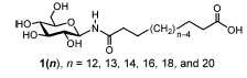
Figure 1: asymmetric bola lipid family, a large, glucose-based hydrophilic group connected by a hydrocarbon chain to a small hydrophilic group
Unfortunately, it appears the molecule you are interested in, is not a glycolipid as published but has a different connectivity. You need to implement this molecule yourself! However, you may use existing building blocks as much as possible. Below, we explain how to go about this.
The first step is therefore to split the molecule in reasonable building blocks. This is sometimes referred to as a mapping (from atomistic to coarse-grained representations). If you consider the chemical nature of the molecular fragments and the existing Martini models for glycolipids and proteins, you may come up with an 8-bead model for the molecule with a linker of 12 C-atoms (n=12 in Figure 1). It may be useful to make a drawing showing which atoms you group into which bead, showing the bead type, as in e.g. the Martini glycolipid paper cited above. A reasonable mapping based on the glycolipid GCER is shown in Figure 2. GCER is representative of both glucosyl- and galactosylceramide; the structures can be found in more detail also on the lipid library website. Although GCER has an amide group, it is connected via an ether linker in GCER, whereas it is directly attached to the sugar ring in our lipid, so we will need to come up with different bond and angle parameters, but the mapping scheme seems reasonable.
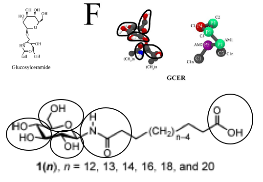
Figure 2: Published glycolipid GCER and possible (partial) mapping of asymmetric bola lipid family
Let us call the new molecule GDAL (for glucose-dodecane-acid-lipid). You can probably think of a much better name, but this is the name that will be assumed in the following...
You will need to write a topology file for the molecule. You may start from scratch, or you may take an existing file and edit it. A good candidate may be the GCER lipid. GCER itself is just the name of the head group linked to a ceramide; if we look in the Martini lipidome, we find a ceramide lipid, DPGS, with two tails, that may well be useful as a template. Some part of the .itp file is shown here:
[ moleculetype ]
DPGS 1
[ atoms ]
1 P4 1 DPGS C1 1 0 72.0000
2 P1 1 DPGS C2 2 0 72.0000
3 P1 1 DPGS C3 3 0 72.0000
4 P1 1 DPGS AM1 4 0 72.0000
5 P5 1 DPGS AM2 5 0 72.0000
6 C3 1 DPGS D1A 6 0 72.0000 ; corrected (C3 instead of C1), oct 2013
7 C1 1 DPGS C2A 7 0 72.0000
8 C1 1 DPGS C3A 8 0 72.0000
9 C1 1 DPGS C4A 9 0 72.0000
10 C1 1 DPGS C1B 10 0 72.0000
11 C1 1 DPGS C2B 11 0 72.0000
12 C1 1 DPGS C3B 12 0 72.0000
13 C1 1 DPGS C4B 13 0 72.0000
Based on other lipid mappings and the connectivity lower down in the file, and the drawing in Figure 2, beads 1-3 are the glucose ring particles, bead 4 is the connection to the glycerol parent of the lipid, bead 5 is the amide, and the other beads are the tails. We should connect bead 5 to bead 3 instead of bead 4 as is done in DPGS, then keep the tail connected to bead 5, which are beads 10-13. Based on 12 CH2-groups, the original bead 13 will be the carboxylic acid end bead. This means all assignments can stand, except that for bead 13, which instead of C1 should probably best be P3. This assignment is based on the Martini 2007 paper, where P3 is representative of acetic acid. So, the first step is to copy the DPGS file, rename DPGS to GDAL, remove beads 4-9, change the type of bead 13 from C1 to P3 and renumber the remaining beads. Before renumbering, perhaps it is best to remove all lines in the [ bonds ], [ angles ], and [ dihedrals ] sections that involve the original beads 4-9. Now the renumbering can be done by changing all entries 5 to 4, 10 to 5, etc. Automatically, the bonded parameters are preserved. There is one thing we need to fix, and that is the bonded parameters around the old bead 5, the new bead 4. The ring bead-amide distance, and ring bead-amide-hydrocarbon angle should be given reasonable values. What are these? The moiety itself is fairly rigid, so the angle around the amide is likely something like 180 degrees, with reasonably high force constant. The ring bead-amide distance may be close to the backbone-backbone distance in proteins. You can look these up in the Martini publications.
Now you have a topology. You can download also the coordinates for DPGS, remove beads 4-9 and use those coordinates for a minimization in vacuum. This coordinate file can then be used to partly fill an empty simulation volume with randomly placed molecules. Water may be added, 10% of the water may be made into anti-freeze water, and a self-assembly simulation may be run as in the lipid tutorial. Follow the protocol shown there.
If you've done all that, you may want to have a look at how one of us did it by downloading this archive. 200 molecules certainly like to form a bilayer, but it does not appear all that bent, maybe because the different head groups not separated on the different sides of the amphiphile layer as proposed by Masuda and Shimizu. This may again be due to the limited number of molecules, the periodic boundary conditions and/or some of the parameters, or much longer relaxation times being required to allow the lipids to flip-flop. This is where the fun starts! You are free to change interaction strengths one level up or down, which means you could test different bead assignments. It may be useful to check whether a single molecule in water has the correct flexibility by running an atomistic simulation and performing the mapping. A similar procedure is shown below for toluene and elsewhere in the lipid and polymer tutorials. Have fun!
Parametrizing a new molecule based on atomistic simulations
In this part of the tutorial I'll explain how to create a Martini topology for a molecule that has not been parametrized before. The procedure is highly dependent on the chemical structure of the molecule and what (experimental) data is available for your molecule. In this example we use a small molecule, toluene, for which an atomistic topology and water-octanol partitioning data (LogP) is available (2.73 from http://dx.doi.org/10.1021/ci050282s). The tutorial assumes you have general experience with the Martini force field (if not, try the other tutorials on this webpage), experience with Gromacs (if not, check the Gromacs-pages and th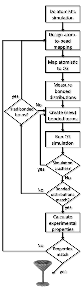 e tutorials mentioned there) and experience with a text editor.
1) Generate atomistic reference data. For most reliable parametrization, atomistically simulate the molecule in solution. Martini has mostly been based on Gromos, but you can use any force field you like. If no topology exists you could use the ATB or the GAFF force field to construct one (this might be quite some work as well). Alternatively, if other people have published results with atomistic resolution for the molecule in question, you may rely on this data as reference material.
The choice of solvent is of importance: The molecule might behave differently in aqueous or apolar solvents and the CG model might not be able capture both equally well. Choose a solvent comparable to the environment where the molecule will spend most of its time. If both environments are important, you may choose to compromise and get the best of two worlds.
For toluene you can run the simulations using (click on the files to download):
grompp -f gromos.mdp -c gromos.gro -p gromos.top -o gromos
mdrun -v -deffnm gromos
This lets you do a simulation of a single toluene molecule in decane as a solvent. Notice that the 1 ns simulation time used in the example is enough because toluene is such a simple molecule.
2) Choose an atom-to-bead mapping. This is the heart of "Coarse Graining" and relies on experience, chemical knowledge and trial-and-error. My favorite method: Draw your molecule on paper, copy it 10 times and start drawing and trying: It's just like primary school. There are no hard rules but here are some tips you could use:
- You have to use the beads in Table 3 from the original Martini paper. Find chemical sub-structures in your molecule that match the example fragments in that table. Don't worry about bonds/angles/dihedrals between the beads yet.
- Split the molecule in blocks of aproximately 4 heavy atoms. For planar or ring structures or when 4 atoms simply don't fit use S-beads. Remember that S-beads only have a small radius compared to standard beads and will thus have the same partitioning free energy (between water and octanol) as normal beads. For example one SC3 bead in P4 solvent (water) will behave exactly as a C3 would.
- Don't use partial charges. Except for fully charged molecules, Martini beads are neutral (exceptions could be made for strongly delocalized charges as found in metal ligands, for instance). For charges use the 'Q'-type beads.
- Compare to existing Martini topologies. Your molecule might contain chemical structures that do not appear in Table 3. But maybe someone else already tackled that problem, for example in proteins, sugars, etc.
- Respect the symmetry of the molecule, and use the same beads for the same chemical groups within one molecule.
3) Coarse-grain target atomistic data. Using your just created mapping, reverse transform the simulation you did at 1) to CG resolution. There are many ways to do this: you can use the reverse transformation tool or use initram.sh. However, in my opinion the simplest method is to create a Gromacs index file where every index group stands for a bead and contains the mapped atom numbers. For toluene run:
seq 0 2 | g_traj -f gromos.xtc -s gromos.gro -oxt mapped.xtc -n mapping.ndx -com -ng 3
where 3 is the number of CG beads in your molecule and the 'seq 0 2' avoids having to type all index groups. Inspect the file mapping.ndx to see how the atoms of toluene are grouped into the CG beads.
4) Generate target CG distributions. Go back to the drawing table and identify between which beads there should be bonded interactions (bonds, constraints, angles, proper and improper dihedrals). Measure the length/angle of these interactions in you mapped-to-CG atomistic simulations from step 3 (mapped.xtc). To do this, create a index file with a directive for "[bonds]" containing (multiple) pairs of CG beads, "[angles]" containing triples and "[dihedrals]" quartets. Use g_bond for the bonds, g_angle for angles and dihedrals:
g_bond -f mapped.xtc -n bonded.ndx -noaver -d
g_angle -f mapped.xtc -n bonded.ndx -ov angles.xvg -type angle -all
From the generated files, create histograms (in the g_angle output the first dataset is the average and can be discarded). You can use g_analyze. e.g. for the angles:
g_analyze -f angles.xvg -dist angledistr.xvg -bw 1.
In some cases it might be sufficient to calculate the average and standard deviation for all the distributions, however the distributions might be bimodal and it is always wise to inspect the distributions! Using xmgrace for the angle distributions, type:
xmgrace -nxy -dist angledistr.xvg
A word of warning is in order here. You may see strange bond distributions if your mapped molecule is split by the periodic boundary conditions. To remedy this, you can first convert your atomistic trajectory to make molecules whole (trjconv -pbc whole) and then do the mapping. Another thing to beware of is that the g_bond command shown above does give average and standard deviation of the separate bonds in the list in the index file in the output file bonds.log, but only the average value is plotted in the file distance.xvg. To get separate distributions for the different bonds, you either need to run g_bond for each bond separately, or follow the procedure shown below for the CG trajectory. Once you have a CG .tpr file, you can run the CG procedure also on the mapped trajectory and have a direct comparison of bond length distributions.
5) Create the CG itp file. This has to be done by hand, although some copy-pasting from existing itp files might help to get the format right. The different directives you (probably) need are:
- "[ moleculetype ]": One line containing the molecule name and a number of exclusions. For Martini the standard is 1.
- "[ atoms ]" One line per atom, containing atomnumber, beadtype, residuenumber, residuename, atomname, chargegroup, charge. Residue number and residue name will be all the same for small molecules. Atomname can be freely chosen. In Martini every bead has its own charge group. Charge can be 0,1 or -1. Mass is not specified and taken from the bead definition.
- "[ bonds ]" One line per bond, containing atom 1, atom 2, function, average length, force constant. The functional form for Martini is 1. Bond length can be set to the average length obtained in step 4. The force constant should be adjusted to the width of the obtained histograms: small width means high force constant and visa versa.
- "[ constraints ]", "[ angles ]", "[ dihedrals ]", see the gromacs manual for the right format.
6) Create CG simulation. Extract one frame from your mapped trajectory and solvate it in the same solvent as the atomistic simulation. Create a top file (include the general martini itp files and the newly created molecule itp and add the right number of molecules (solute and solvent)). Create a Martini mdp file (see examples on the website). Simulate the initial form of the CG molecule (you probably will have to energy minimize and maybe relax for a few thousand steps at a smaller timestep (e.g. 5fs). You also need itp, itp and itp. It may be wise to create a separate directory for the CG system.
grompp -f em.mdp -c martini.gro -p martini.top -o em
mdrun -v -deffnm em
grompp -f relax.mdp -c em.gro -p martini.top -o relax
mdrun -v -deffnm relax
grompp -f md.mdp -c relax.gro -p martini.top -o md
mdrun -v -deffnm md
In this simulation measure the bonded interactions similar to what you did in step 4 for the mapped trajectory. You can use the same index file.
g_bond -f md.xtc -s md.tpr -n bonded.ndx -noaverdist -d bonds_martini.xvg
g_angle -f md.xtc -n bonded.ndx -ov angles_martini.xvg -type angle -all
Note the difference on the g_bond command compared to the treatment of the mapped trajectory. Here, you add a directive for the tpr file (-s md.tpr) and set -noaverdist.
7) Optimize CG bonded parameters. In step 6 two things might happen: The simulation finishes and you obtain distributions or the simulation crashes. In the first case, you can compare the distributions to the ones obtained in step 4 and go back to step 5 to adjust the parameters in the itp to obtain better distributions. Too wide distributions mean you'll need higher force constants, averages being off means you need to shift, etc. If the simulation crashes you will also have to go back to step 5, now with the aim to make the molecule more stable. This often means lowering force constants, removing uncessesary dihedrals or changing constraints to bonds or vice versa. Some common source of instability are:
- If a (proper) dihedral is defined over 4 atoms and the angle between 3 atoms is very wide (close to 180 degrees) this may lead to heavy fluctuations and crashes. You'll might have to remove the dihedral or use special types of dihedrals.
- In ring like structures beads might be connected in triangles. If constraints are used between those beads, LINCS might not be able to solve them.
- Three beads, a,b and c, are linearly connected with short, weak bonds, bead b will be excluded from a and c. If a and c strongly attrack each other, a or c might start overlapping with b.
Repeat until you're happy with the result, then move to the last step.
8) Compare to experimental results. Partitioning free energies (we are currently working on a tutorial explaining how to efficiently calculate those for Martini molecules) are particularly good, but for pure liquids also densities can be used or any other experimental number you can lay your hands on.
Martini workshop lectures
- Details
-
Last Updated: Friday, 11 August 2017 06:55
MARTINI WORKSHOP 2017, Groningen, The Netherlands
Monday, August 21
Introduction to the Martini model, Siewert Jan Marrink slides
Lipid biophysics with the Martini model, Helgi Ingólfsson slides
Tuesday, August 22
Martini model for proteins, Alex de Vries slides
Peptide aggregation, Pim Frederix slides
Photosystem II, Floris van Eerden slides
Wednesday, August 23
TOOLS: martinize, martinate, insane, backward, daft, Tsjerk Wassenaar slides
Advanced parameterization of Martini, Manuel Nuno Melo slides
Multiscaling with Martini, Manuel Nuno Melo slides
Thursday, August 24
The Martini model for DNA and RNA, Ignacio Faustino Plo slides
Blends for organic photovoltaics, Riccardo Alessandri slides
The future of Martini, Paulo Telles de Souza slides
MARTINI WORKSHOP 2015, Groningen, The Netherlands
Monday, August 24
Introduction to coarse-graining, Alex de Vries slides
Introduction to the Martini model, Siewert Jan Marrink slides
Tuesday, August 25
Lipid biophysics with the Martini model, Helgi Ingólfsson slides
Martini model for proteins, Alex de Vries slides
Wednesday, August 26
TOOLS: martinize, martinate, insane, backward, daft, Tsjerk Wassenaar slides
Martini model for saccharides (includes also other polymers and dna), Siewert Jan Marrink slides
Thursday, August 27
Advanced parameterization of Martini, Manuel Nuno Melo slides
Multiscaling with Martini, Manuel Nuno Melo slides
Martini flowchart
- Details
-
Last Updated: Tuesday, 25 August 2015 20:39
You have a (bio)molecular system you want to simulate at coarse-grain level
yes
|
no
Does your system contain proteins/peptides?
yes
|
no
Does your system contain lipids (and possibly cholesterol)?
yes
|
no
Does your system contain:
Check
this page for a more exhaustive list of parameterized compounds.
|
no
|
... and others!
nope, everything's covered
You might want to constrain the secondary structure of your protein.
Are electrostatic interactions likely to be important?
yes
|
no
You can use the
martinize.py script to build protein topologies.
One good thing done.
Does it contain only simple lipids (such as DPPC, DOPE, POPC, etc.) or cholesterol?
yes
|
not only
Does it contain
glycolipids?
yes
|
no
Does it contain sphingolipids?
yes
|
no
You can build your system using the
insane.py script.
Was easy after all, wasn't it?
Martini tutorials: visualization
- Details
-
Last Updated: Sunday, 20 August 2017 09:19
Martini tutorials: visualizing Martini systems using VMD
VMD is a molecular visualization program for displaying, animating, and analyzing large biomolecular systems using 3-D graphics and built-in scripting. (http://www.ks.uiuc.edu/Research/vmd/).
In this module, we explain some of the vmd commands that can be used to visualize the CG systems. Additionally, Tcl scripts are presented that assist with the visualization of CG systems; these scripts, as well as extended help, are available on the Martini website:
http://md.chem.rug.nl/cgmartini/index.php/tools2/visualization
An additional, very usefull tool for displaying CG (Martini) structures in VMD is Bendix. A good tutorial for Bendix can be found here:
http://sbcb.bioch.ox.ac.uk/Bendix/
Some basics
VMD adopted a representation-philosophy: for any set of atoms/molecules/protein chains we want to display or analyze, we need to select this set through a "representation" de�fined by keywords related to this set (somewhat similar to make_ndx). VMD comes with implemented keywords for all-atom systems ("protein", "chain", "hydrogen", "solvent", etc.). More general keywords are implemented to be able to display non-classical-systems (CG systems are part of this second category); you can fi�nd them in VMD manual:
http://www.ks.uiuc.edu/Research/vmd/current/ug/
Below are listed a few examples:
- To select only lipids: resname POPC, or only part of each lipids: resname POPC and name "C.*.A" "C.*.*.B" "D.*.A" "D.*.B" for lipid tails (C1A,C1B, etc.) and resname POPC and name NC3 PO4 "GL.*" for heads.
- To select only backbone beads of a protein: name BB (use "BB.*" or BAS for old versions of FG-to-CG scripts).
- To get rid of solvent (water/ion beads): not resname W WF ION or WP in case of polarizable water.
- To show only charged positively charged residues (in Martini): resname LYS ARG.
- To display the water shell around specifc residues: within 7.0 of (index 531 to 538).
- To display all lipids (excluding DPPC) whose heads are interacting with the same speci�fic residues: same resid as ((within 7.0 of (index 531 to 538)) and name NC3 PO4 "GL.*") and not resname DPPC.
As you can see in the examples, all these keywords can be mixed with the logical links: and, or, not, etc. to produce any representation. Try it yourself! VMD is really demanding in term of memory; an easy trick to decrease the amount needed by VMD is to load structure/trajectories containing only beads needed by your analysis; this can easily be done by preprocessing the trajectory using trjconv. And as we are simulating bigger and bigger systems in which more and more beads are involved, the previous trick can be adapted to increase the displaying/seeking speed of trajectories by writing representations showing only beads needed for the visualization (head groups of a bilayer for instance). Keep in mind that you can save the visualizing state of your system whenever you want by saving a state.vmd �file. This �file contains the Tcl commands needed to obtain the current display; lists of bonds and drawings (cylinders) are not saved, but you can open this .vmd file and manually add the lines you wrote to generate them at the bottom.
CG bonds/constraints and elastic networks
When a CG structure/trajectory is opened with VMD, the program builds a network of bonds using a distance criteria and an atomistic library of possible bond lengths (de�ned by the namd force field, developed by the same group); CG beads, linked with bonds with an average length of 0.35 nm, are not de�fined through this automatic algorithm. VMD inevitably ends up displaying a cloud of dots, which are hard (impossible?) to properly visualize with non-bionic human eyes. A Tcl script which reads the bonds and constraints from the CG .itp/.tpr files, and rewrites the CG bond network is available on the Martini website.
First, make sure your system knows where to �find the script:
source /wherever/cg_bonds.tcl
This script can now be used from the command line window of VMD as follows:
cg_bonds -top system.top -topoltype "elastic"
in case you have a .top available, but no gromacs. Alternatively, if gromacs is installed on the machine you are using, you may use a .tpr instead:
cg_bonds -gmx /wherever/gmxdump -tpr dyn.tpr -net "elastic" -cutoff� 12.0 -color "orange"
-mat "AOChalky" -res 12 -rad 0.1
The last line will draw the ElNeDyn network with the options (cuto�ff, color, material, resolution and radius) speci�ed by extracting the bonds from the dyn.tpr �file (that's where the gmxdump comes in). Note that you must specify a my gromacs version compatible with the dyn.tpr �file.
Visualization of secondary structure
After being able to draw bonds and constraints de�ned by the CG force�eld, the next step is to see protein secondary structure. We are currently developing a graphical script drawing vmd cartoon-like representation. This set of routines is still under development, and needs to be improved. . . by your feedback?
Two main routines are provided by the cg_secondary_structure.tcl script: cg_helix and cg_sheet.
Use these two commands in the same fashion:
cg_whatever {list of terminig} [-graphical options]
Or, in an example:
cg_helix {{5 48} {120 146}} -hlxmethod "cylinder" -hlxcolor "red" -hlxrad 2.5
which will draw two helices, from residue labeled as 5 to residue labeled as 48 and from residue labeled as 120 to residue labeled as 146, as red cylinder of radius 0.25 nm. Check the help shown when the script is sourced or the website for an exhaustive list of options and default values. To defi�ne the list of termini, two options are implemented: i) providing the list by yourself (like in the example shown above), ii) reading/parsing a �file generated by do_dssp. In the second case, you don't need to provide any termini, but the list of termini still needs to be written in the command line as an empty list: {}.
Please keep in mind that, due to the restricted amount of structural information carried on by a CG structure, the beauty and exactitude of these graphical representations are limited. . .
Martini Workshops
- Details
-
Last Updated: Monday, 12 July 2021 09:03
Martini Workshops
Upcoming workshops
Groningen, The Netherlands 2021 (online workshop)
Past workshops
Groningen, The Netherlands 2017 (full)
Groningen, The Netherlands 2015
Lausanne, Switzerland 2011
Levi, Finland 2010
Helsinki, Finland 2009
Education resources
- Details
-
Last Updated: Friday, 02 October 2015 12:37
You can learn more about different aspects of Martini in three ways:
- On your own using our tutorials: visit the tutorials page here.
- By participating to a Martini workshop: check the next availability here.
- Learn about getting specialized assistance here.
Polarizable Water
- Details
-
Last Updated: Thursday, 22 August 2013 09:00
Polarizable water
In this part of the tutorial we will convert water in an existing Martini-system to polarizable water. In the polarizable Martini paper* the model is described as follows:
"The polarizable CG water consists of three particles instead of one in the standard Martini force �eld. The central particle W is neutral and interacts with other particles in the system by means of the Lennard-Jones interactions, just like the standard water particle. The additional particles WP and WM are bound to the central particle and carry a positive and negative charge of +0.46 and -0.46, respectively. They interact with other particles via a Coulomb function only, and lack any LJ interactions. The bonds W-WP and W-WM are constrained to a distance of 0:14nm. The interactions between WP and WM particles inside the same CG water bead are excluded, thus these particles are "transparent" toward each other. As a result the charged particles can rotate around the W particle. A harmonic angle potential with equilibrium angle phi = 0 rad and force constant Kh = 4.2 kJ mol-1 rad-2 is furthermore added to control the rotation of WP and WM particles and thus to adjust the distribution of the dipole momentum."
If you want to solvate a new system with polarizable water, follow the steps in the protein part of the Martini tutorial, section 6. Instead of a normal waterbox and .mdp/.itp fi�les use the waterbox containing polarizable water and polarizable Martini .mdp and .itp fi�les (available from the Martini website: http://cgmartini.nl). Note that minimizing a polarizable Martini system requires some tweaking, as described below.
If you have an existing system with normal Martini water and want to change to polarizable water you may use the python script triple-w.py. For this example we convert dppc_bilayer.gro/dppc_bilayer.top available here.
1. Create a new gro �file:
triple-w.py dppc_bilayer.gro
The python-script triple-w.py adds positive and negative sites at a small distance to every central water bead in a .gro �file.
2. Adapt the .top file. Make sure the polarizable version of the particle defi�nition martini_v2.P.itp fi�le is included. In the .mdp file the value of epsilon_rc has to be adapted and the index group W renamed into PW (Download an example here). The .itp �files for the lipids and possibly other molecules do not have to be changed.
3. If polarizable water is used in combination with proteins or peptides, all AC1 and AC2 beads have to be replaced by normal C1 and C2 beads. AC1 and AC2 are obsolete in polarizable Martini.
4. Minimize the system. For polarizable water to minimize without problems, it is SOMETIMES necessarry to change the constraints to stiff� bonds. Using the ifdef-statement in the martini v2.P.itp fi�le, this can be set using a de�fine value in the .mdp fi�le (have a look at the bottom of martini v2.P.itp to see how it works).
5. Set the correct options in martini_v2.P_example.mdp (e.g. "integrator = steep", "nsteps = 50", "constraints = none", "epsilon_r = 2.5", etc.) and the "defi�ne" option to -DEM and change the W index group name.
6. Generate the input fi�les for the minimization run:
grompp -f martini v2.P example.mdp -c dppc-polW.gro -p dppc bilayer.top -o em -maxwarn 1
7. Proceed with equilibration and production runs.
*S.O. Yesylevskyy, L.V. Schäfer, D. Sengupta, S.J. Marrink, Polarizable Water Model for the Coarse-Grained MARTINI Force Field, PLoS Comput. Biol. 6, e1000810, 2010
Reverse transformation
- Details
-
Last Updated: Thursday, 22 August 2013 08:59
Reverse transformation
In this module we explore the use of the reverse-transformation tool, to convert between coarse-grained and fine-grained representations of a system.
Simulations at coarse-grained level allow the exploration of longer time-scales and larger length-scales than at the usual atomistic level. However, the loss of detail can seriously limit the questions that can be asked to the system. Methods that re-introduce atomic details in a CG structure are therefore of considerable interest. Such structures provide starting points in phase space for simulations at the more detailed level that may otherwise take too long to reach. As a demonstration of such a method, we will use restrained simulated annealing (SA) to increase the resolution of a system containing a WALP peptide spanning a DPPC bilayer. We will investigate how the number of steps allowed for the reconstruction influences the quality of the generated FG structure.
Reverse transformation: transformation run
In this part of exercise we will use a modi�ed version of gromacs that allows one to generate a FG structure from CG beads*. The same version is also used to transform a FG structure to CG beads, section 1e. Thus, the program allows one to switch between FG and CG representations. To achieve this, additional information is put in the topology �le at the FG level in a section called [ mapping ]. The tool pdb2gmx can generate this mapping for proteins automatically. Note that this will usually require the option -missing to be speci�ed! Two new functions in mdrun are responsible for restrained simulated annealing (SA) to converge from a random FG structure to a FG structure compatible with the CG structure, i.e. the FG positions are optimized in such a way that the CG structure is preserved in the FG-to-CG mapping (each CG bead is at the center of mass of the FG atoms that map to it). There is also small tool, called g_fg2cg, to generate CG structures from FG ones defi�ned by the mapping and random FG starting structures based on CG input �le, that are afterwards optimized during a SA run.
The source code for this version of the script can be found Downloads/Tools section of this website.
The files needed for this section can be downloaded from:
rev_trans.tar.gz
Transformation run
1. Unpack the rev_trans.tar.gz in the MARTINITUTORIAL directory that contains all necessary gromacs �files for this exercise.
2. Compile and/or source the modifi�ed version of gromacs (remember this tool is based upon gromacs version 3.3.1 and needs the corresponding tricks and threats to be compiled.)
source /where-ever-you-installed-it/gromacs-3.3.1/bin/GMXRC
export GMXLIB=/where-ever-you-installed-it/gromacs-3.3.1/share/gromacs/top
3. Modify the FG fg.top fi�le in such a way that the number of water and lipid molecules is the same as in the coarse-grained model. One FG_W corresponds to four normal water molecules.
4. Use g_fg2cg to construct an input atomistic structure for a simulated annealing run. The coarse grain structure is already prepared for you and is called cg.gro. Check the output with ngmx or VMD.
g_fg2cg -pfg fg.top -pcg dppc_cg.top -n 0 -c cg.gro -o fg.gro
5. Use grompp to create a topol.tpr �file.
6. Perform a SA run by typing
mdrun -coarse cg.gro -v
7. Change the number of simulation steps to 1000 and SA time parameters to 0 1.5 0 1.5 0 1.5 in your mdp file. (see comments for additional mdp options at the bottom of fg.mdp �file) Perform another SA run with the altered parameters.
8. Change the number of simulation steps to 5000 and SA time parameters to 0 7.5 0 7.5 0 7.5. Perform a SA run again.
9. If you have enough time, change the number of simulation steps to 60000 and SA time parameters to 0 100 0 100 0 100. Repeat the SA run.
10. Plot the potential energies for all runs and compare them.
11. Compare FG WALP models from all runs. Check secondary structure and phi� and psi angles.
12. Compare dihedral distribution for one of dihedral angles from the tail of the DOPC lipids.
*A.J. Rzepiela, L.V. Schäafer, N. Goga, H.J. Risselada, A.H. de Vries, S.J. Marrink, Reconstruction of atomistic detail from coarse grained structures, J. Comput. Chem., 31, 1333-1343 (2010)
Bilayer tutorial
- Details
-
Last Updated: Thursday, 22 August 2013 08:56
Bilayer system setup
The aim of the first part is to create and study properties of coarse-grained models of lipid bilayer membranes. First, we will attempt to spontaneously self-assemble a DSPC bilayer and check various properties that characterize lipid bilayers, such as the area per lipid, bilayer thickness, P2 order parameters, and diffusion. Next, we will change the nature of the lipid head groups and tails, and study how that influences the properties. Finally, there is a slightly more advanced exercise on how to parameterize a Martini CG model of diC18:2-PC, a PC lipid with a doubly unsaturated tail, based on an all-atom simulation.
The files for the first section can be downloaded here:
lipid_tutorial.tar.gz
Unpack the lipid-tutorial.tar.gz archive (it expands to a directory called lipid-tutorial).
We will begin with self-assembling a DSPC (distearoyl-phosphatidylcholine) bilayer from a random configuration of lipids and water in the simulation box. Enter the spontaneous-assembly subdirectory; first, create this random configuration of 128 DSPC starting from a single DSPC molecule:
genbox -ci dspc_single.gro -nmol 128 -box 7.5 7.5 7.5 -try 500 -o 128_noW.gro
Next, minimize the system...
grompp -f em.mdp -c 128_noW.gro -p dspc.top -maxwarn 10
mdrun -v -c 128_minimised.gro
...add 6 CG waters (i.e., 24 all-atom waters) per lipid...
genbox -cp 128_minimised.gro -cs water.gro -o waterbox.gro -maxsol 768 -vdwd 0.21
The value of the flag -vdwd (default van der Waals radii) has to be increased from its default atomistic length (0.105 ns) to a value reflecting the size of Martini coarse-grained beads.
...and minimize again (adapt dspc.top to reflect the water beads added to the system):
grompp -f em.mdp -c waterbox.gro -p dspc.top -maxwarn 10
mdrun -v -c minimised.gro
Bilayer self-assembly
Now, you are ready to run the self-assembly MD simulation. About 25 ns should suffice.
grompp -f md.mdp -c minimised.gro -p dspc.top -maxwarn 10
mdrun -v
This might take ca. 45 min on a single CPU. If you have a parallel version of gromacs installed, issue "mpirun -np 2 mdrun -rdd 1.4 -v" to run a job on 2 CPUs. You may want to check the progress of the simulation to see whether the bilayer has already formed before the end of the simulation. You may do this most easily by starting the inbuilt GROMACS viewer:
ngmx
or, alternatively, use VMD. In the meantime, have a close look at the Martini parameter files; in particular, the interactions and bead types. What are the differences between PC and PE head groups as well as between saturated and unsaturated tails?
Check whether you got a bilayer. If yes, check if the formed membrane is normal to the z-axis (i.e., membrane in the xy-plane). If the latter is not the case, rotate the system accordingly (with editconf). In case you did not get a bilayer at all, continue with the pre-formed one from “dspc_bilayer.gro”. Set up a simulation for another 15 ns at zero surface tension (switch to semiisotropic pressure coupling) at a higher temperature of 341 K. This is above the experimental gel to liquid-crystalline transition temperature of DSPC. You will find how to change pressure coupling and temperature in the GROMACS manual:
http://manual.gromacs.org/current/
Again, you may not want to wait for this simulation to fi�nish. In that case, you may skip ahead and use a trajectory provided in the subdirectory bilayer-analysis/dspc .
Bilayer analysis
From the latter simulation, we can calculate properties such as
- area per lipid
- bilayer thickness
- P2 order parameters of the bonds
- lateral diffusion of the lipids
In general, for the analysis, you might want to discard the first few ns of your simulation (equilibration time).
Area per lipid
To get the (projected) area per lipid, you can simply divide the area of your simulation box (Box-X times Box-Y from g_energy) by half the number of lipids in your system. (Note that this might not be strictly OK, because the self-assembled bilayer might be slightly asymmetric in terms of number of lipids per monolayer, i.e., the areas per lipid are different for the two monolayers. However, to a first approximation, we will ignore this here.)
Bilayer thickness
To get the bilayer thickness, use g_density. You can get the density for a number of different functional groups in the lipid (e.g., phosphate and ammonium headgroup beads, carbon tail beads, etc) by feeding an appropriate index-file to g_density (make one with make_ndx; you can select, e.g., the phosphate beads by typing “a P*”). The bilayer thickness you can obtain from the distance between the headgroup peaks in the density profile.
A more appropriate way to compare to experiment is to calculate the electron density profile. The g_density tool also provides this option. However, you need to supply the program with a data-file containing the number of electrons associated with each bead (option -ei electrons.dat). The format is described in the GROMACS manual.
Compare your results to those from small-angle neutron scattering experiments (Balgavy et al., Biochim. et Biophys. Acta 2001, 1512, 40-52):
- thickness = 4.98 ± 0.15 nm
- area per lipid = 0.65 ± 0.05 nm2
Lateral diffusion
Before calculating the lateral diffusion, remove jumps over the box boundaries (trjconv -pbc nojump). Then, calculate the lateral diffusion using g_msd. Take care to remove the overall center of mass motion (-rmcomm*), and to fit the line only to the linear regime of the mean-square-displacement curve (-beginfit and -endfit options of g_msd). To get the lateral diffusion, choose the ”-lateral z” option.
To compare the diffusion coefficient obtained from a Martini simulation to a measured one, a conversion factor of about 4 has to be applied to account for the faster diffusion at the CG level due to the smoothened free energy landscape.
*In GROMACS 3, this option is not available. An additional “trjconv -center” will do the trick.
Order parameters
Now, we will calculate the (second-rank) order parameter, which is defined as
P
2
= 1/2 (3 cos2<θ> − 1) ,
where θ is the angle between the bond and the bilayer normal. P2 = 1 means perfect alignment with the bilayer normal, P2 = −0.5 anti-alignment, and P2 = 0 random orientation.
The newest version of the script to calculated these order parameters can be downloaded here (there is also a version located in the subdirectory bilayer-analysis/scripts). Copy the .xtc and .tpr �les in the bilayer-analysis/dspc subdirectory (should be named traj.xtc and topol.tpr, respectively; you may want to use the 30 ns simulations already present there instead). The script do-order.py will calculate P2 for you. As it explains when you invoke it, it needs a number of arguments. The command:
> ./do-order.py 0 10000 20 0 0 1 64 DSPC
will for example read in a 10 ns trajectory of 64 DSPC lipids and average over 20 equally-spaced snapshots. P2 is calculated relative to the z-axis.
Changing lipid type
Lipids can be thought of as modular molecules. In this section, we investigate the eff�ect of changes in the lipid tails and in the headgroups on the properties of lipid bilayers using the Martini model. We will i) introduce a double bond in the lipid tails, and ii) change the lipid head groups from PC to PE.
Unsaturated tails
To introduce a double bond in the tail, we will replace the DSPC lipids by DOPC (compare the Martini topologies of these two lipids). Replace DSPC by DOPC in your .top and .mdp files, and grompp will do the rest for you (you can ignore the ”atom name does not match” warnings of grompp).
Changing the headgroups
Starting again from the final snapshot of the DSPC simulation, change the head groups from PC to PE. For both new systems, run 15-ns MD simulations and compare the above properties (area per lipid, thickness, order parameter, diffusion) between the three bilayers (DSPC, DOPC, DSPE). Do the observed changes match your expectations? Why/why not? Discuss.
Refine lipid parameters
This section uses the fi�ne-grained-to-coarse-grained (FG-to-CG) transformation tool, which is treated in a later section of the Martini tutorial. If you are unfamiliar with the tool, you might want to skip this section fi�rst and continue with the rest of the tutorial.
In this part, we will try to obtain improved Martini parameters for diC18:2-PC, a PC lipid with a doubly unsaturated tail. We will try to optimise the Martini parameters such that the dihedral and angle distributions within the lipid tail match those from a 100 ns all-atom simulation (all-atom data in “fg.xtc”) as close as possible. The files needed in this section are located in the "refine" directory.
The task can be divided into the following five steps:
- Transform the all-atom (fine-grained, FG) trajectory into its coarse-grained counterpart, based on a pre-defined mapping scheme*.
- Calculate the angle and dihedral distributions. These will serve as the reference (“gold standard”) later.
- Do a coarse-grained simulation of the system.
- Calculate the angle and dihedral distibutions, and compare to the reference.
- Revise coarse-grained parameters, repeat steps 3 and 4 until you are satisfied with the result.
*The mapping is already defined, look at the [mapping] section in dupc_fg.itp
For the transformation from FG to CG, we will use the program g_fg2cg, which is part of a modified version of GROMACS that you need to install yourself (see section "3: Reverse transformation"):
source /where-ever-your-installation-is/bin/GMXRC
setenv GMXLIB /where-ever-your-installation-is/share/top
First, transform from FG to CG:
g_fg2cg -pfg fg.top -pcg cg.top -c fg.gro -n 1 -o cg.gro
g_fg2cg -pfg fg.top -pcg cg.top -c fg.xtc -n 1 -o fg2cg.xtc
Then, make an index file needed for the calculation of the angle and dihedral distributions within the lipid tail:
make_ndx -f cg.gro -o angle.ndx
aGL1 | aC1A | aD2A
aC1A | aD2A | aD3A
aD2A | aD3A | aC4A
aC1A | aD2A | aD3A | aC4A
q
Now, calculate the distributions with g_angle:
g_angle -f fg2cg.xtc -type angle -n angle.ndx -od fg2cg ang{1,2,3}.xvg g_angle -f fg2cg.xtc -type dihedral -n angle.ndx -od fg2cg dih1.xvg
These are the target distributions that we want to obtain with the CG model. As a starting point, we will use the Martini parameters as defined in “dupc_cg.itp”, i.e., all angles at 180 degrees. Carry out a short CG simulation (starting from “cg_mdstart.gro”, you just have to add water to the cg.top). (Don't forget to source a regular version of Gromacs!) You will need to make an appropriate .mdp �le. Note that the FG trajectory was obtained at a temperature of 300 K.After comparing the angle and dihedral distributions to the fg2cg reference, change the angle parameters in “dupc_cg.itp” and repeat.
Proteins
- Details
-
Last Updated: Thursday, 22 August 2013 08:59
Protein in water
Keeping in line with the overall Martini philosophy, the coarse-grained protein model groups 4 heavy atoms together in one CG bead. Each residue has one backbone bead and zero or more side-chain beads depending on the amino acid type. The secondary structure of the protein influences both the selected bead types and bond/angle/dihedral parameters of each residue as explained below. It is noteworthy that, even though the protein is free to change its tertiary arrangement, local secondary structure is predefi�ned and thus imposed throughout a simulation. Conformational changes that involve changes in the secondary structure are therefore beyond the scope of Martini CG proteins.
Setting up a CG protein simulation consists basically of two steps:
1. converting an atomistic protein structure into a CG model;
2. generating a suitable Martini topology.
Both steps are done using the publicly available 'martinize.py' script, of which the latest version can be downloaded here.
The aim of this module is to set up a CG simulation of ubiquitin in a water box. In this part of the tutorial, some basic knowledge of gromacs commands is assumed and not all commands will be given explicitly. Please refer to the previous tutorials and/or the gromacs manual. After getting the atomistic structure of ubiquitin (1UBQ), you'll need to convert it into a CG structure and to prepare a Martini topology for it. Once this is done the CG structure can be minimized, solvated and simulated. The steps you need to take are roughly the following:
1. Download 1UBQ.pdb from the Protein Data Bank.
wget http://www.rcsb.org/pdb/files/1UBQ.pdb.gz
gzip -d 1UBQ.pdb.gz
2. The pdb-structure can be used directly as input for the martinize.py script, to generate both a structure and a topology file. Have a look at the help function (i.e. run martinize.py -h) for the available options. Hint: During equilibration it might be useful to have (backbone) position restraints. The fi�nal command might look a bit like this:
./martinize.py -f 1UBQ.pdb -o system.top -x cg_1UBQ.pdb
                  -dssp /wherever/dsspcmbi -p backbone -ff martini22
When using the -dssp option you'll need the dssp binary, which determines the secondary structure classification of the protein backbone from the PDB-structure. It can be downloaded from a CMBI website:
As an alternative, you may prepare a fi�le with the required secondary structure yourself and feed it to the script:
./martinize.py -f 1UBQ.pdb -o system.top -x cg_1UBQ.pdb
-ss your-sec-struct-fi�le -p backbone -ff martini22
NOTE: The martinize.py script might not work with older versions of python! Also python 3.x migth not work. We know it does work with versions: [2.6.x, 2.7.x] and does not work with [2.4.x]. If you have tested it with any version inbetween, we would like to hear from you.
3. If everything went well, the script generated three �files: a coarse grain structure (.gro/.pdb), a master topology �file (.top), and a protein topology file (.itp). In order to run a simulation you need two more: the Martini topology �file (martini v2.1.itp) and a run parameter �le (.mdp). You can get examples from the Martini website or from the protein-tutorial package. Don't forget to adapt the settings where needed!
4. Do a short (+/-10 steps!) minimization in vacuum. (Before you can generate the run-input �files with grompp, you have to generate a box, for example using editconf).
5. Solvate the system with genbox (an equilibrated water box can be downloaded here) and minimize. Make sure the box-size is large enough (i.e. there is enough water around the molecule) and remember to use a larger van der Waals distance when solvating to avoid clashes, e.g.:
genbox -cp confout.gro -cs water-1bar-303K.gro -vdwd 0.21 -o solvated.gro
6. Do a short energy minimization and position restrained simulation. Since the martinize.py script already generated position restraints (thanks to the -p option), all you have to do is specify
de�fine = -DPOSRES
in your .mdp �file and add the appropriate number of water (W) beads to your .top fi�le.
7. Start production run (without position restraints!).
8. . . .
9. PROFIT! What sort of analysis can be done on this molecule? Start by having a look at the protein with vmd (section Visualizing Martini systems using vmd).
A mapped fine-grained simulation of ubiquitin for comparison is available in the archive mapubq.tar.gz
Protein and elastic network
The aim of this module is to see how application of elastic networks can be combined with the Martini model to conserve tertiary and quartenary structures more faithfully without sacri�cing realistic dynamics of a protein. We o�ffer two alternative routes. Please be advised that this is an active �field of research and that there is as of yet no "gold standard". The �first option is to generate a simple elastic network on the basis of a standard Martini topology. The second options is to use an ElNeDyn network. This second option constitutes quite some change to the Martini forcefi�eld and thus is a di�fferent forcefi�eld! The advantage is that the behavior of the method has been well described*. Both approaches can be set up using the martinize.py script and will be shortly described below.
First you should simulate a normal Martini CG protein without an elastic network and then see what changes when you use a CG topology with an elastic network.
1. Download HIV-1 Protease (1A8G.pdb).
2. Repeat steps 2-7 from the previous exercise. (You'll need to simulate the protein for hundreds of nanoseconds to see major changes in the structure, a sample long simulation is provided in the archive 1A8G_trajectories.tar.gz).
3. Visualize the simulation; look especially at the binding pocket of the protein: does it stay closed, open up, or what? What happens to the overall protein structure?
Martini + elastic network
The �first option to help preserve higher-order structure of proteins is to add to the standard Martini topology extra harmonic bonds between non-bonded beads based on a distance cut-o�ff. Note that in standard Martini, long harmonic bonds are already used to impose the secondary structure of extended elements (sheets) of the protein. The martinize.py script will generate harmonic bonds between backbone beads if the options -elastic is set. It is possible to tune the elastic bonds (e.g.: make the force constant distance dependent, change upper and lower distance cut-off�, etc.) in order to make the protein behave properly. The only way to �f8nd the proper parameters is to try di�fferent options and compare the behavior of your protein to an atomistic simulation or experimental data (NMR, etc.). Here we will use basic parameters in order to show
the principle.
1. Use the martinize.py script to generate the coarse grain structure and topology as above. For the elastic network options use:
-elastic -ef 500 -el 0.5 -eu 0.9 -ea 0 -ep 0
This turns on the elastic network (-elastic), sets the elastic bond force constant to 500 kJ mol-1 nm-2 (-ef 500), the lower and upper elastic bond cut-o� to 0.5 and 0.9 nm, respectively, (-el 0.5 -eu 0.9) and makes the bond strengths independent of the bond length (elastic bond decay factor and decay power, -ea 0 -ep 0, respectively; these are default). The elastic network is defi�ned in the .itp fi�le by an "ifdef" statement (have a look!). The "#defi�ne RUBBER BANDS" in the .top or .itp �file switches it on. Note that martinize.py does not generate elastic bonds between i->i+1 and i->i+2 backbone bonds, as those are already connected by bonds and angles.
2. Proceed as before and start a production run. If you are using a Gromacs version older then 4.5.x you have to explicitly set the "define = -DRUBBER_BANDS" in the mdp-file. In 4.5.x and further this is automatically set in the top file.
ElNeDyn
The second option to use elastic networks in combination with Martini puts more emphasis on remaining close to the overall structure as deposited in the PDB than standard Martini does. The main di�fference from the standard way (used in the previous exercise) is the use of a global elastic network between the backbone beads to conserve the conformation instead of relying on the
angle/dihedral potentials and/or local elastic bonds to do the job. The position of the backbone beads is also slightly di�erent. In standard Martinithe center-of-mass of the peptide plane is used as the location of the backbone bead, but in the elastic network implementation the positions of the C�-atoms are used for this.
The martinize.py script automatically sets these options and sets the correct parameters for the elastic network. As the elastic bondstrength and the upper cut-off� have to be tuned in an ElNeDyn network, these options can be set manually (-ef -eu).
1. Use the martinize.py script to generate the coarse grain structure and topology as above. Set the following options (-ef 500 and -eu 0.9 are the default options, so can be left away):
-elnedyn -ef 500 -eu 0.9
This selects the ElNeDyn topology options, with a force constant of 500 kJ mol-1nm-2 (-ef 500) and an upper bond length cut-o� of 0.9 nm (-eu 0.9).
2. Proceed as before and start a production run.
Now you've got three simulations of the same protein with diff�erent elastic networks. If you do not want to wait, some pre-run trajectories can be found in: 1A8G_trajectories.tar.gz One of them might fi�t your needs in terms of structural and dynamic behavior. If not, there are an almost in�nite number of ways to further tweak the elastic network!
An easy way to compare the slightly di�erent behaviors of the proteins in the previous three cases is to follow deviation/fluctuation of the backbone during simulation (and compare it to an all-atom simulation if possible). vmd provides a set of friendly tools to compute RMSD/RMSF, but it needs some tricks to be adapted to CG systems ("protein", "water", etc. keywords are not understood by vmd on CG structures). In this specifi�c case, to visualize/select only the backbone you need to create a representation containing only the corresponding beads: "name BB". See section on Coarse Grain vizualization for more detailed howtos and advice.
*X. Periole, M. Cavalli, S.J. Marrink, M.A. Ceruso, Combining an Elastic Network With a Coarse-Grained Molecular Force Field: Structure, Dynamics, and Intermolecular Recognition, J. Chem. Theory Comput., 5, 2531-2543 (2009)