


- Details
- Last Updated: Thursday, 22 August 2013 08:56
Bilayer system setup
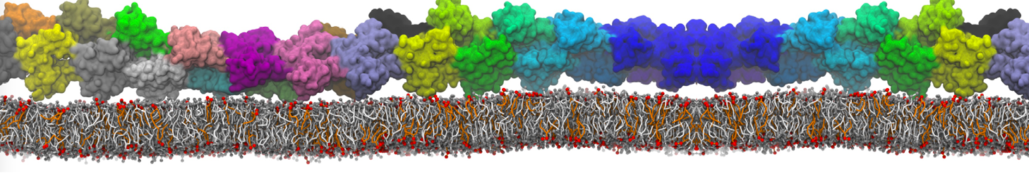
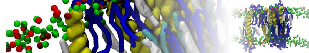
The aim of the first part is to create and study properties of coarse-grained models of lipid bilayer membranes. First, we will attempt to spontaneously self-assemble a DSPC bilayer and check various properties that characterize lipid bilayers, such as the area per lipid, bilayer thickness, P2 order parameters, and diffusion. Next, we will change the nature of the lipid head groups and tails, and study how that influences the properties. Finally, there is a slightly more advanced exercise on how to parameterize a Martini CG model of diC18:2-PC, a PC lipid with a doubly unsaturated tail, based on an all-atom simulation.
The files for the first section can be downloaded here:
lipid_tutorial.tar.gzUnpack the lipid-tutorial.tar.gz archive (it expands to a directory called lipid-tutorial).
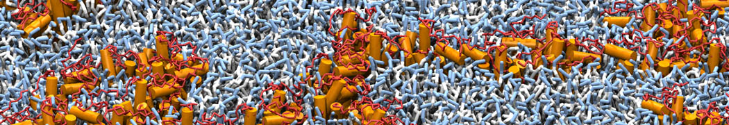
We will begin with self-assembling a DSPC (distearoyl-phosphatidylcholine) bilayer from a random configuration of lipids and water in the simulation box. Enter the spontaneous-assembly subdirectory; first, create this random configuration of 128 DSPC starting from a single DSPC molecule:
genbox -ci dspc_single.gro -nmol 128 -box 7.5 7.5 7.5 -try 500 -o 128_noW.gro
Next, minimize the system...
grompp -f em.mdp -c 128_noW.gro -p dspc.top -maxwarn 10
mdrun -v -c 128_minimised.gro
...add 6 CG waters (i.e., 24 all-atom waters) per lipid...
genbox -cp 128_minimised.gro -cs water.gro -o waterbox.gro -maxsol 768 -vdwd 0.21
The value of the flag -vdwd (default van der Waals radii) has to be increased from its default atomistic length (0.105 ns) to a value reflecting the size of Martini coarse-grained beads.
...and minimize again (adapt dspc.top to reflect the water beads added to the system):
grompp -f em.mdp -c waterbox.gro -p dspc.top -maxwarn 10
mdrun -v -c minimised.gro
Bilayer self-assembly
Now, you are ready to run the self-assembly MD simulation. About 25 ns should suffice.
grompp -f md.mdp -c minimised.gro -p dspc.top -maxwarn 10
mdrun -v
This might take ca. 45 min on a single CPU. If you have a parallel version of gromacs installed, issue "mpirun -np 2 mdrun -rdd 1.4 -v" to run a job on 2 CPUs. You may want to check the progress of the simulation to see whether the bilayer has already formed before the end of the simulation. You may do this most easily by starting the inbuilt GROMACS viewer:
ngmx
or, alternatively, use VMD. In the meantime, have a close look at the Martini parameter files; in particular, the interactions and bead types. What are the differences between PC and PE head groups as well as between saturated and unsaturated tails?
Check whether you got a bilayer. If yes, check if the formed membrane is normal to the z-axis (i.e., membrane in the xy-plane). If the latter is not the case, rotate the system accordingly (with editconf). In case you did not get a bilayer at all, continue with the pre-formed one from “dspc_bilayer.gro”. Set up a simulation for another 15 ns at zero surface tension (switch to semiisotropic pressure coupling) at a higher temperature of 341 K. This is above the experimental gel to liquid-crystalline transition temperature of DSPC. You will find how to change pressure coupling and temperature in the GROMACS manual:
http://manual.gromacs.org/current/Again, you may not want to wait for this simulation to fi nish. In that case, you may skip ahead and use a trajectory provided in the subdirectory bilayer-analysis/dspc .
Bilayer analysis
From the latter simulation, we can calculate properties such as
- area per lipid
- bilayer thickness
- P2 order parameters of the bonds
- lateral diffusion of the lipids
In general, for the analysis, you might want to discard the first few ns of your simulation (equilibration time).
Area per lipid
To get the (projected) area per lipid, you can simply divide the area of your simulation box (Box-X times Box-Y from g_energy) by half the number of lipids in your system. (Note that this might not be strictly OK, because the self-assembled bilayer might be slightly asymmetric in terms of number of lipids per monolayer, i.e., the areas per lipid are different for the two monolayers. However, to a first approximation, we will ignore this here.)
Bilayer thickness
To get the bilayer thickness, use g_density. You can get the density for a number of different functional groups in the lipid (e.g., phosphate and ammonium headgroup beads, carbon tail beads, etc) by feeding an appropriate index-file to g_density (make one with make_ndx; you can select, e.g., the phosphate beads by typing “a P*”). The bilayer thickness you can obtain from the distance between the headgroup peaks in the density profile.
A more appropriate way to compare to experiment is to calculate the electron density profile. The g_density tool also provides this option. However, you need to supply the program with a data-file containing the number of electrons associated with each bead (option -ei electrons.dat). The format is described in the GROMACS manual.
Compare your results to those from small-angle neutron scattering experiments (Balgavy et al., Biochim. et Biophys. Acta 2001, 1512, 40-52):
- thickness = 4.98 ± 0.15 nm
- area per lipid = 0.65 ± 0.05 nm2
Lateral diffusion
Before calculating the lateral diffusion, remove jumps over the box boundaries (trjconv -pbc nojump). Then, calculate the lateral diffusion using g_msd. Take care to remove the overall center of mass motion (-rmcomm*), and to fit the line only to the linear regime of the mean-square-displacement curve (-beginfit and -endfit options of g_msd). To get the lateral diffusion, choose the ”-lateral z” option.
To compare the diffusion coefficient obtained from a Martini simulation to a measured one, a conversion factor of about 4 has to be applied to account for the faster diffusion at the CG level due to the smoothened free energy landscape.
*In GROMACS 3, this option is not available. An additional “trjconv -center” will do the trick.
Order parameters
Now, we will calculate the (second-rank) order parameter, which is defined as
P
2
= 1/2 (3 cos2<θ> − 1) ,
where θ is the angle between the bond and the bilayer normal. P2 = 1 means perfect alignment with the bilayer normal, P2 = −0.5 anti-alignment, and P2 = 0 random orientation.
The newest version of the script to calculated these order parameters can be downloaded here (there is also a version located in the subdirectory bilayer-analysis/scripts). Copy the .xtc and .tpr les in the bilayer-analysis/dspc subdirectory (should be named traj.xtc and topol.tpr, respectively; you may want to use the 30 ns simulations already present there instead). The script do-order.py will calculate P2 for you. As it explains when you invoke it, it needs a number of arguments. The command:
> ./do-order.py 0 10000 20 0 0 1 64 DSPC
will for example read in a 10 ns trajectory of 64 DSPC lipids and average over 20 equally-spaced snapshots. P2 is calculated relative to the z-axis.
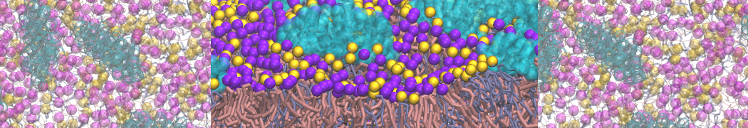
Changing lipid type
Lipids can be thought of as modular molecules. In this section, we investigate the eff ect of changes in the lipid tails and in the headgroups on the properties of lipid bilayers using the Martini model. We will i) introduce a double bond in the lipid tails, and ii) change the lipid head groups from PC to PE.
Unsaturated tails
To introduce a double bond in the tail, we will replace the DSPC lipids by DOPC (compare the Martini topologies of these two lipids). Replace DSPC by DOPC in your .top and .mdp files, and grompp will do the rest for you (you can ignore the ”atom name does not match” warnings of grompp).
Changing the headgroups
Starting again from the final snapshot of the DSPC simulation, change the head groups from PC to PE. For both new systems, run 15-ns MD simulations and compare the above properties (area per lipid, thickness, order parameter, diffusion) between the three bilayers (DSPC, DOPC, DSPE). Do the observed changes match your expectations? Why/why not? Discuss.
Refine lipid parameters
This section uses the fi ne-grained-to-coarse-grained (FG-to-CG) transformation tool, which is treated in a later section of the Martini tutorial. If you are unfamiliar with the tool, you might want to skip this section fi rst and continue with the rest of the tutorial.
In this part, we will try to obtain improved Martini parameters for diC18:2-PC, a PC lipid with a doubly unsaturated tail. We will try to optimise the Martini parameters such that the dihedral and angle distributions within the lipid tail match those from a 100 ns all-atom simulation (all-atom data in “fg.xtc”) as close as possible. The files needed in this section are located in the "refine" directory.
The task can be divided into the following five steps:
- Transform the all-atom (fine-grained, FG) trajectory into its coarse-grained counterpart, based on a pre-defined mapping scheme*.
- Calculate the angle and dihedral distributions. These will serve as the reference (“gold standard”) later.
- Do a coarse-grained simulation of the system.
- Calculate the angle and dihedral distibutions, and compare to the reference.
- Revise coarse-grained parameters, repeat steps 3 and 4 until you are satisfied with the result.
*The mapping is already defined, look at the [mapping] section in dupc_fg.itp
For the transformation from FG to CG, we will use the program g_fg2cg, which is part of a modified version of GROMACS that you need to install yourself (see section "3: Reverse transformation"):
source /where-ever-your-installation-is/bin/GMXRC
setenv GMXLIB /where-ever-your-installation-is/share/top
First, transform from FG to CG:
g_fg2cg -pfg fg.top -pcg cg.top -c fg.gro -n 1 -o cg.gro
g_fg2cg -pfg fg.top -pcg cg.top -c fg.xtc -n 1 -o fg2cg.xtc
Then, make an index file needed for the calculation of the angle and dihedral distributions within the lipid tail:
make_ndx -f cg.gro -o angle.ndx
aGL1 | aC1A | aD2A
aC1A | aD2A | aD3A
aD2A | aD3A | aC4A
aC1A | aD2A | aD3A | aC4A
q
Now, calculate the distributions with g_angle:
g_angle -f fg2cg.xtc -type angle -n angle.ndx -od fg2cg ang{1,2,3}.xvgg_angle -f fg2cg.xtc -type dihedral -n angle.ndx -od fg2cg dih1.xvg
These are the target distributions that we want to obtain with the CG model. As a starting point, we will use the Martini parameters as defined in “dupc_cg.itp”, i.e., all angles at 180 degrees. Carry out a short CG simulation (starting from “cg_mdstart.gro”, you just have to add water to the cg.top). (Don't forget to source a regular version of Gromacs!) You will need to make an appropriate .mdp le. Note that the FG trajectory was obtained at a temperature of 300 K.After comparing the angle and dihedral distributions to the fg2cg reference, change the angle parameters in “dupc_cg.itp” and repeat.