


Martini tutorials: lipids
- Details
- Last Updated: Thursday, 19 May 2016 15:05
Martini tutorials: lipids
Summary
Advanced: Dry Martini and vesicles
Advanced: refine lipid parameters
Tools and scripts used in this tutorial
Lipid bilayers
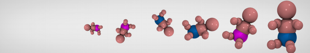
The Martini course-grained (CG) model was originally developed for lipids[1,2]. The underlying philosophy of Martini is to build an extendable CG model based on simple modular building blocks and to use only few parameters and standard interaction potentials to maximise applicability and transferability. Martini uses an approximate 4:1 atomistic (heavy atoms) to CG bead mapping and in version 2.0[2] 18 bead types were defined to represent chemical characteristics of the beads. The CG beads have a fixed size and interact using an interaction map with 10 different interaction strengths. Due to the modularity of Martini, a large set of different lipid types has been parameterized e.g. the Martini lipid topology section.
These tutorials assume a basic understanding of the Linux operating system and the gromacs molecular dynamics (MD) simulation package. An excellent gromacs tutorial available at: md.chem.rug.nl/~mdcourse/.
The aim of the tutorial is to create and study properties of CG Martini models of lipid bilayer membranes. First, we will attempt to spontaneously self-assemble a DSPC bilayer and check various properties that characterize lipid bilayers, such as the area per lipid, bilayer thickness, order parameters, and diffusion. Next, we will change the nature of the lipid head groups and tails, and study how that influences the properties. Finally, we will move on to creating more complex multicomponent bilayers.
Download all the files of this tutorial: bilayer_tutorial.zip Unpack the lipid-tutorial.tar.gz archive (it expands to a directory called bilayer-tutorial).
Bilayer self-assembly
We will begin with self-assembling a distearoyl-phosphatidylcholine (DSPC) bilayer from a random configuration of lipids and water in the simulation box. Enter the spontaneous-assembly subdirectory; first, create a random configuration of 128 DSPC lipids starting from a single DSPC molecule:
$ genbox -ci dspc_single.gro -nmol 128 -box 7.5 7.5 7.5 -try 500 -o 128_noW.gro
Next, minimize the system...
$ grompp -f minimization.mdp -c 128_noW.gro -p dspc.top -maxwarn 10 -o dspc-min-init.tpr
$ mdrun -deffnm dspc-min-init -v -c 128_minimised.gro
...add 6 CG waters (i.e., 24 all-atom waters) per lipid...
$ genbox -cp 128_minimised.gro -cs water.gro -o waterbox.gro -maxsol 768 -vdwd 0.21
The value of the flag -vdwd (default van der Waals radii) has to be increased from its default atomistic length (0.105 nm) to a value reflecting the size of Martini CG beads.
...and minimize again (adapt dspc.top to reflect the water beads added to the system):
$ grompp -f minimization.mdp -c waterbox.gro -p dspc.top -maxwarn 10 -o dspc-min-solvent.tpr
$ mdrun -deffnm dspc-min-solvent -v -c minimised.gro
Now, you are ready to run the self-assembly MD simulation. About 25 ns should suffice.
$ grompp -f martini_md.mdp -c minimised.gro -p dspc.top -maxwarn 10 -o dspc-md.tpr
$ mdrun -deffnm dspc-md -v
This might take ca. 45 min on a single CPU but by default mdrun will use all available CPUs on your machine. You can tune the numbers of parallel threads mdrun uses with the -nt parameter. You may want to check the progress of the simulation to see whether the bilayer has already formed before the end of the simulation. You may do this most easily by starting the inbuilt gromacs viewer:
$ ngmx -f dspc-md.xtc -s dspc-md.tpr
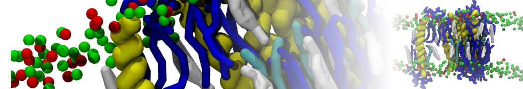
or, alternatively, use VMD, the inital and final snapshots should look similar to Fig. 1. In the meantime, have a close look at the Martini parameter files; in particular, the interactions and bead types. What are the differences between PC and PE headgroups as well as between saturated and unsaturated tails?
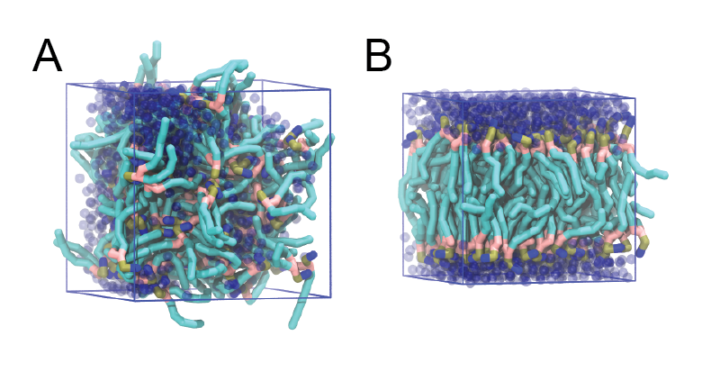
Figure 1 | DSPC bilayer formation. A) 64 randomly localized DSPC lipid molecules with water. B) After a 30 ns long simulation the DSPC lipids have aggregated together and formed a bilayer.
Check whether you got a bilayer. If yes, check if the formed membrane is normal to the z-axis (i.e., membrane in the xy-plane). If the latter is not the case, rotate the system accordingly (with editconf). In case you did not get a bilayer at all, continue with the pre-formed one from dspc_bilayer.gro. Set up a simulation for another 15 ns at zero surface tension (switch to semiisotropic pressure coupling) at a higher temperature of 341 K. This is above the experimental gel to liquid-crystalline transition temperature of DSPC. You will find how to change pressure coupling and temperature in the gromacs manual: manual.gromacs.org/current/online.html Again, you may not want to wait for this simulation to finish. In that case, you may skip ahead and use a trajectory provided in the subdirectory spontaneous-assembly/allfiles/.
Bilayer analysis
From the latter simulation, we can calculate properties such as:
- area per lipid
- bilayer thickness
- P2 order parameters of the bonds
- lateral diffusion of the lipids
In general, for the analysis, you might want to discard the first few ns of your simulation as equilibration time.
Area per lipid
To get the (projected) area per lipid, you can simply divide the area of your simulation box (Box-X times Box-Y from g_energy) by half the number of lipids in your system. (Note that this might not be strictly OK, because the self-assembled bilayer might be slightly asymmetric in terms of number of lipids per monolayer, i.e., the areas per lipid are different for the two monolayers. However, to a first approximation, we will ignore this here.)
Bilayer thickness
To get the bilayer thickness, use g_density. You can get the density for a number of different functional groups in the lipid (e.g., phosphate and ammonium headgroup beads, carbon tail beads, etc) by feeding an appropriate index-file to g_density (make one with make_ndx; you can select, e.g., the phosphate beads by typing a P*). The bilayer thickness you can obtain from the distance between the headgroup peaks in the density profile.
A more appropriate way to compare to experiment is to calculate the electron density profile. The g_density tool also provides this option. However, you need to supply the program with a data-file containing the number of electrons associated with each bead (option -ei electrons.dat). The format is described in the gromacs manual.
Compare your results to those from small-angle neutron scattering experiments[3]:
- thickness = 4.98 ± 0.15 nm
- area per lipid = 0.65 ± 0.05 nm2
Lateral diffusion
Before calculating the lateral diffusion, remove jumps over the box boundaries (trjconv -pbc nojump). Then, calculate the lateral diffusion using g_msd. Take care to remove the overall center of mass motion (-rmcomm*), and to fit the line only to the linear regime of the mean-square-displacement curve (-beginfit and -endfit options of g_msd). To get the lateral diffusion, choose the -lateral z option.
To compare the diffusion coefficient obtained from a Martini simulation to a measured one, a conversion factor of about 4 has to be applied to account for the faster diffusion at the CG level due to the smoothened free energy landscape (note, the conversion factor can vary significantly depending on the molecule in question).
*In gromacs v3, this option is not available. An additional trjconv -center will do the trick.
Order parameters
Now, we will calculate the (second-rank) order parameter, which is defined as:
P2 = 1/2 (3 cos2<θ> − 1),
where θ is the angle between the bond and the bilayer normal. P2 = 1 means perfect alignment with the bilayer normal, P2 = −0.5 anti-alignment, and P2 = 0 random orientation.
A script to calculated these order parameters can be downloaded here (there is also a version located in the directory scripts/). Copy the .xtc and .tpr files to a analysis subdirectory (the script expects them to be named traj.xtc and topol.tpr, respectively; you may want to use the 15 ns simulations already present in the subdirectory spontaneous-assembly/allfiles/). The script do-order-multi.py will calculate P2 for you. As it explains when you invoke it, it needs a number of arguments. The command:
$ ./do-order-multi.py traj.xtc 0 15000 20 0 0 1 64 DSPC
will for example read 0 to 15 ns from the trajectory traj.xtc. The simulation has 64 DSPC lipids and the output is the P2, calculated relative to the Z-axis, and average over results from every 20th equally-spaced snapshot in the trajectory.
Additional analysis
Different scientific questions require different methods of analysis and no set of tools can span them all. There are various tools available in the gromacs package, see the gromacs manual: manual.gromacs.org/current/online.html. Most simulation groups, therefore, develop sets of customized scripts and programs many of which they make freely available, such as the Morphological Image Analysis and the 3D pressure field tools available here. Additionally a number of packages are available to for assistance with analysis and the development of customized tools, such as the python MDAnalysis package pypi.python.org/pypi/MDAnalysis/.
Changing lipid type
Lipids can be thought of as modular molecules. In this section, we investigate the effect of changes in the lipid tails and in the headgroups on the properties of lipid bilayers using the Martini model. We will i) introduce a double bond in the lipid tails, and ii) change the lipid headgroups from phosphatidylcholine (PC) to phosphatidylethanolamine (PE).
Unsaturated tails
To introduce a double bond in the tail, we will replace the DSPC lipids by DOPC (compare the Martini topologies of these two lipids - martini_v2.0_lipids.itp). Replace DSPC by DOPC in your .top and .mdp files, and grompp will do the rest for you (you can ignore the ”atom name does not match” warnings of grompp).
Changing the headgroups
Starting again from the final snapshot of the DSPC simulation, change the head groups from PC to PE. For both new systems, run 15 ns MD simulations and compare the above properties (area per lipid, thickness, order parameter, diffusion) between the three bilayers (DSPC, DOPC, DSPE). Do the observed changes match your expectations? Why/why not? Discuss.
Complex bilayer mixtures
When setting up larger and more complex bilayers it can be more convenient, or necessary, to start with a bilayer close to equilibrium rather then trying to get the bilayer to self-assemble. This can be done by concatenating (e.g. using editconf) and/or altering previously formed bilayers or by using a bilayer formation program such as insane.py, available in the directory scripts/ or downloadable here. INSANE (INSert membrANE) is a CG building tool that generates membranes by distributing lipids over a grid. Lipid structures are derived from simple template definitions that can either be added to the program or provided on-the-fly from combinations of headgroup, linker and lipid tails specified on the command-line. The program uses two grids, one for the inner and one for the outer leaflet, and distributes the lipids randomly over the grid cells with numbers according to the relative quantities specified. This allows for building asymmetric bilayers with specific lipid compositions. The program also allows for adding solvent and ions, using a similar grid protocol it distributes them over a 3D grid. Additional information about the functionality of INSANE can be found by running insane.py -h.
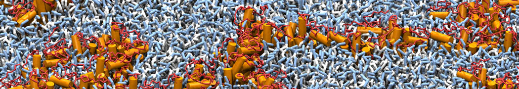
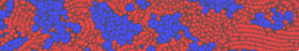
In the directory complex-bilayers/ we will create a fully hydrated 4:3:3 mole ratio bilayer of DPPC:DUPC:CHOL with physiological ion concentration using insane.py, this is a similar mixture as was used in Risselada and Marrink[4] to show raft formation. Start by running INSANE:
$ ./insane.py -l DPPC:4 -l DUPC:3 -l CHOL:3 -salt 0.15 -x 15 -y 10 -z 9 -d 0 -pbc cubic -sol W -o dppc-dupc-chol-insane.gro
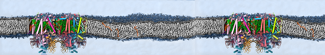
This will generate an initial configuration for the system dppc-dupc-chol-insane.gro (Fig. 2A) and provide initial information of the .top file. Next, fix the .top file by including the correct Martini topologies. Then, energy minimize the structure and run a short (10 ns) equilibrium simulation in a similar manner as explained in the bilayer self-assembly section. Note, as this simulation contains multiple components you will have to make an index file (using make_ndx) and group all the lipids together and all the solvent together to fit the specified groups in the .mdp files. As all the bilayer lipids and solvent were places on a grid (Fig. 2A), even after minimization they can still be in an energetically unfavorable state. Due to the large forces involved it may be necessary to run a few equilibrium simulations using a short time step (1-10 fs) before running production simulations with Martini lipid time steps (30-40 fs). The initial grid order imposed by insane.py should relax in a few ns (Fig. 2B), we recommend simulating for 5-30 ns using the Berendsen pressure coupling algorithm, to relax the membrane area, before switching to Parrinello-Rahman for the production run. This mixture will phase separate at a temperature of 295 K but that can take multiple microseconds (Fig. 2C).
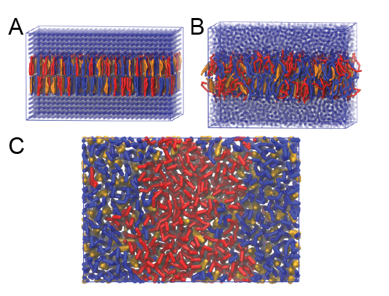
Figure 2 | DPPC-DUPC-CHOL bilayer formation. A) Using insane.py a 4:3:3 DPPC-DUPC-CHOL bilayer was setup. B) After a 20 ns long simulation the grid structure is gone and the bilayer area has equilibrated. C) This lipid mixture phase separates into Ld and Lo domains at 295 K, this phase separation can take multiple microseconds, showing a top view of the simulation after 6 microseconds. In all panels DPPC is in red, DUPC in blue and cholesterol in orange.
Advanced: Dry Martini and vesicles
In this tutorial we are going to study the deformation of a lipid vesicle due to demixing and formation of Lo and Ld phases. To study this type of system composed of a very large number of particles, a specific force field has recently been developed: Dry Martini. This Martini-derived force field, as its name indicates, doesn't require any aqueous solvent and allows the simulation of much larger systems.
The use of this force field requires very specific parameters for production runs; everything is explained in the package found there.
Update: We recommend that you generate your vesicle using the CHARMM-GUI. Follow the tutorial on how to use it here and continue to follow this tutorial after you've equilibrated your vesicle.
-
Generate the vesicle using the martini_vesicle_builder.py script available there. The following command will generate a 25 nm diameter vesicle with randomly distributed DPPC, DUPC (DLiPC) and cholesterol molecules.
$ python martini_vesicle_builder.py 12.5 DPPC:DUPC,60:40 43 1> system.gro 2> system.top
-
Minimize the system.
-
Equilibrate the system. In this case, a long equilibration is required: the vesicle is built based on properties (thickness and area per lipid) extracted from pure flat bilayers; these properties will be drastically modified by the curvature of the vesicle bilayer. Pores will form in the bilayer, but will be quickly closed and help the equilibration (lipid flip-flop) of the vesicle.
-
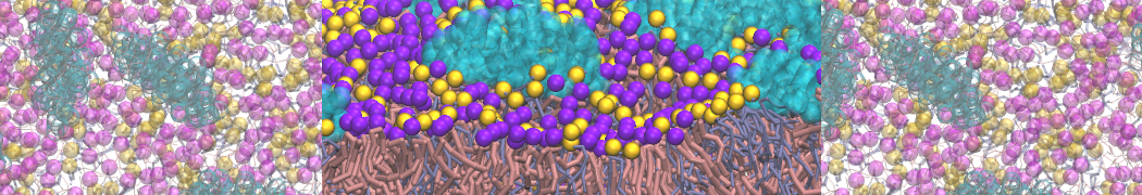
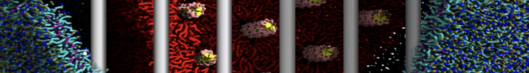
Production run should be at least 10 µs. Check the evolution of the geometry of the system: how is the demixing affecting the sphericity of the vesicle? An example is given in Figure 3.
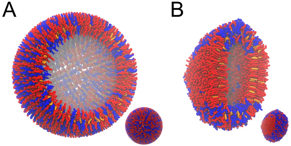
Figure 3 | DPPC-DUPC-CHOL vesicle, ball-to-doughnut transformation. A) Initial system, and B) conformation after a 20 µs long simulation: note the flatten sides of the vesicle, denoting the Lo phases (DPPC/CHOL). The insets are showing the full system, while the bigger snapshots are showing a cut.
Advanced: refine lipid parameters
Warning this section is a few years old and has not been tested recently. Also, this section uses the fine-grained-to-coarse-grained (FG-to-CG) transformation tool, which is treated in a later section of the Martini tutorial. If you are unfamiliar with the tool, you might want to skip this section.
In this part, we will try to obtain improved Martini parameters for diC18:2-PC, a PC lipid with a doubly unsaturated tail. We will try to optimise the Martini parameters such that the dihedral and angle distributions within the lipid tail match those from a 100 ns all-atom simulation (all-atom data in fg.xtc) as close as possible. The files needed in this section are located in the refine/ directory.
The task can be divided into the following five steps:
- Transform the all-atom (fine-grained, FG) trajectory into its coarse-grained counterpart, based on a pre-defined mapping scheme*.
- Calculate the angle and dihedral distributions. These will serve as the reference (“gold standard”) later.
- Do a coarse-grained simulation of the system.
- Calculate the angle and dihedral distibutions, and compare to the reference.
- Revise coarse-grained parameters, repeat steps 3 and 4 until you are satisfied with the result.
*The mapping is already defined, look at the [mapping] section in dupc_fg.itp.
For the transformation from FG to CG, we will use the program g_fg2cg, which is part of a modified version of gromacs that you need to install yourself (see tutorial "Reverse transformation"):
$ source /where-ever-your-installation-is/bin/GMXRC
$ setenv GMXLIB /where-ever-your-installation-is/share/top
First, transform from FG to CG:
$ g_fg2cg -pfg fg.top -pcg cg.top -c fg.gro -n 1 -o cg.gro
$ g_fg2cg -pfg fg.top -pcg cg.top -c fg.xtc -n 1 -o fg2cg.xtc
Then, make an index file needed for the calculation of the angle and dihedral distributions within the lipid tail:
$ make_ndx -f cg.gro -o angle.ndx
aGL1 | aC1A | aD2A
aC1A | aD2A | aD3A
aD2A | aD3A | aC4A
aC1A | aD2A | aD3A | aC4A
q
Now, calculate the distributions with g_angle:
$ g_angle -f fg2cg.xtc -type angle -n angle.ndx -od fg2cg ang{1,2,3}.xvg
$ g_angle -f fg2cg.xtc -type dihedral -n angle.ndx -od fg2cg dih1.xvg
These are the target distributions that we want to obtain with the CG model. As a starting point, we will use the Martini parameters as defined in dupc_cg.itp, i.e., all angles at 180 degrees. Carry out a short CG simulation (starting from cg_mdstart.gro, you just have to add water to the cg.top). (Don't forget to source a regular version of gromacs!) You will need to make an appropriate .mdp. Note that the FG trajectory was obtained at a temperature of 300 K. After comparing the angle and dihedral distributions to the g_fg2cg reference, change the angle parameters in dupc_cg.itp and repeat.
Tools and scripts used in this tutorial
gromacs (http://www.gromacs.org/)
insane.py (downloadable here)
MDAnalysis package (pypi.python.org/pypi/MDAnalysis/0.8.1)
[1] Marrink, S. J., De Vries, A. H., and Mark, A. E. (2004) Coarse grained model for semiquantitative lipid simulations. J. Phys. Chem. B 108, 750–760.
[2] Marrink, S. J., Risselada, H. J., Yefimov, S., Tieleman, D. P., and De Vries, A. H. (2007) The MARTINI force field: coarse grained model for biomolecular simulations. J. Phys. Chem. B 111, 7812–7824.
[3] Balgavy, P., Dubnicková, M., Kucerka, N., Kiselev, M. A., Yaradaikin, S. P., and Uhrikova, D. (2001) Bilayer thickness and lipid interface area in unilamellar extruded 1,2-diacylphosphatidylcholine liposomes: a small-angle neutron scattering study. Biochim. Biophys. Acta 1512, 40–52.
[4] Risselada, H. J., and Marrink, S. J. (2008) The molecular face of lipid rafts in model membranes. Proc. Natl. Acad. Sci. U.S.A. 105, 17367–17372.