Parametrization of a new small molecule using Fast_Forward
Contributed by: @csbrasnett, @ricalessandri.
In case of issues, please contact Chris Brasnett or open an issue on the repo.Summary
IntroductionGenerate atomistic reference dataAtom-to-bead mappingGenerate the CG mapped trajectory from the atomistic simulationCreate the initial CG itp and tpr filesGenerate target CG distributions from the CG mapped trajectoryCreate the CG simulationOptimize CG bonded parametersComparison to experimental results, further refinements, and final considerationsTools and scripts used in this tutorialReferences
Introduction
In this tutorial, we will discuss how to build a Martini 3 topology for a new small molecule using a semi-automated method with the Fast_Forward Python package. This tutorial builds on ideas and techniques discussed in the classic Small Molecule Parameterization tutorial [1,2], and it is recommended that you do that tutorial before this one.
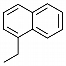
As before, we will use as an example the molecule 1-ethylnaphthalene (Fig. 1), and make use of Gromacs versions 2024.x or later. Files for this tutorial can be found here.
1. Generate atomistic reference data
Here, we will use the SwissParam server [3] as a way to obtain an atomistic (or all-atom, AA) structure and molecule topology based on the Charmm36 force field, but of course feel free to use your favorite atomistic force field.
The previous tutorial used LigParGen to obtain reference topologies. It may be instructive to investigate how the results obtained in parameterization here are different to that one.
Start by feeding the SMILES string for 1-ethylnaphthalene (namely, CCc1cccc2ccccc21) to the SwissParam server. After submitting the molecule, the server will generate input parameters for several molecular dynamics (MD) packages. Download the resulting zip file. You can now unzip the zip archive provided:
unzip files-m3-parametrize_new_small_molecule.zipwhich contains a folder called ENAP-in-water that contains some template folders and useful scripts. We will assume that you will be carrying out the tutorial using this folder structure and scripts. Note that the archive contains also a folder called ENAP-worked where you will find a worked version of the tutorial (trajectories not included). This might be useful to use as reference to compare your files (e.g., to compare the ENAP_LigParGen.itp you obtained with the one you find in ENAP-worked/1_AA-reference).
We can now move to the first subfolder, 1_AA-reference, and copy over the files you just obtained from the LigParGen server:
cd ENAP-in-water/1_AA-reference[move here the obtained zip file from the SwissParam server.]
Input files obtained from SwissParam come with a default residue name of LIG. For now, this does not particularly matter, but it may be useful to change it for record keeping or future reference.
Now launch the AA MD simulation:
bash generate_atomistic_reference.shThe last command will run an energy-minimization, followed by an NPT equilibration of 250 ps, and by an MD run of 10 ns (inspect the script and the various .mdp files to know more). Note that 10 ns is a rather short simulation time, selected for speeding up the current tutorial. You should rather use at least 50 ns, or an even longer running time in case of more complex molecules (you can try to experiment with the simulation time yourself!). In this case, the solvent used is water; however, the script can be adapted to run with any other solvent, provided that you input also an equilibrated solvent box. You should choose a solvent that represents the environment where the molecule will spend most of its time. Finally, a solvent-free trajectory is generated to use for mapping purposes later.
2. Atom-to-bead mapping
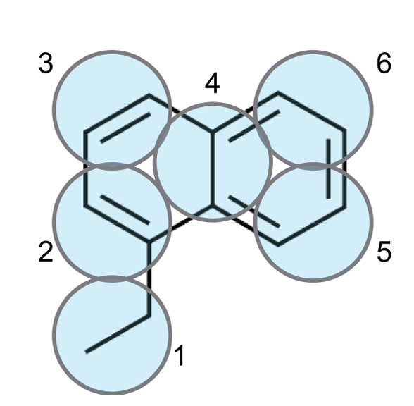
Following the rules set out in the classic Small Molecule Parameterization tutorial, the molecule can be mapped to 6 T-beads, as shown in Fig. 2 below:
3. Generate the CG mapped trajectory from the atomistic simulation
Using the mapping you just created, you will now transform the simulation you did at section 1 to CG resolution using a file in the .map format.
The CGbuilder tool can generate such a file, as it did with the index-based approach in the previous tutorial [4]. Load the lig.gro generated in the previous step, and assign each of the atoms to its corresponding bead in the viewer.
You can now try to map the trajectory using a .map file from CGBuilder. Once done, download the cgbuilder.map file that CGbuilder creates to the 2_mapping folder.
cd ../2_mapping/download cgbuilder.map and move it to the current folder, i.e., ‘2_mapping’
The header of CGbuilder .map files doesn’t quite align with what we exactly need for fast_forward. Make sure the first two lines of the file read as:
[ molecule ]
LIG ENAP
These lines define the name of the molecule at atomistic (LIG) and CG (ENAP) resolution.
You can now run the script:
bash 2_mapping.shwhich will:
- Make a python virtual environment and install the fast forward package in it.
- Use the
ff_mapprogram offast_forwardto map the ligand-only trajectory generated in the previous step.
Note that running ff_map on a trajectory file automatically generates both the mapped trajectory and a single initial frame. Note in the mapped.gro file generated the residue name is now ENAP, having been defined in the .map file above.
4. Generating an initial CG topology
As before, the first goal of parameterisation is to match the bonded parameters at the CG level to the ones mapped from our atomistic simulation. Using the same bonded network as before, generate an initial topology (i.e. ENAP_initial.itp) file for the molecule containing directives for atoms, bonds, dihedrals, virtual_sitesn, and exclusions.
4.1 Using fast_forward to generate initial parameters
One of the powerful features of fast_forward is the ff_inter (interactions) program, which can generate best guess parameters for a CG topology file from an initial input topology and a mapped trajectory.
The initial input topology can be readily adapted from the file that we’ve just generated. Two additional considerations are:
- All interactions (bonds, angles, dihedrals, etc) need to be annotated with an interaction group name
- Bonds may be left as bonds only,
ff_interwill automatically convert high force constants to constraints.
The first interactions directive of the file can then look something like this:
[bonds]
; i j funct length kb
 1 2 1 0.300 5000 ; C1_R1
 1 4 1 0.300 5000 ; C1_R4
 2 3 1 0.300 5000 ; R2_R3
…
[ dihedrals ]
; i j k l func ref.angle force_const
 1 3 6 5 2 0 10 ; C1_R3_R6_R5
…
Note as well that the initial guesses here are completely arbitrary. Any interaction will be analysed ab initio with new parameters calculated.
To run ff_inter we also need a reference .tpr file for the molecule on its own:
gmx grompp -f initial.mdp -p topol.top -c ../2_mapping/mapped.gro -o mapped.tpr -maxwarn 1The ff_inter program can then be invoked with the following command:
ff_inter -f ../2_mapping/mapped.xtc -s mapped.tpr -i ENAP_initial.itp -dists -plots -itp-onlyHere, the mapped trajectory and associated topology (mapped.xtc and mapped.tpr respectively) are analysed using the interactions notated in the input molecule topology file (ENAP_initial.itp). Using the -dists flag writes out time series and histogram data for each of the interactions. The histograms are all also plotted in a figure using the -plots flag: a file called distribution_plots.png is written. For each interaction, the histogram of the interaction data is plotted along with the fit the program has made. Finally, the -itp-only flag indicates that strictly only the interactions notated in the input file should be determined. Otherwise, ff_inter will attempt to generate all possible angles and dihedrals for the molecule from its bonded structure, a feature of the program which may be useful for slightly larger or more flexible molecules.
The program will generate a new itp file based on the molecule name (i.e. ENAP.itp). Compare the input and the output file. The output file should now contain both bonds and constraints, with some bonds separated by an #ifdef statement for energy minimisation purposes, and written in the constraints directive with the inverse statement. The bond lengths and force constants should now be more ‘optimised’ for an initial simulation, with respect to the distributions calculated and shown in the figure generated.
5. Create the CG simulation
We can now finalize the first take on the CG model, ENAP_take1.itp, where we can use the info contained in the data_bonds.txt and data_dihedrals.txt files to come up with better guesses for the bonded parameters:
cd ../4_CG_simcp ../3_initial_CG/ENAP.itp .bash run_CG.shwhere the command will run an energy-minimization, followed by an NPT equilibration, and by an MD run of 100 ns (inspect the script and the various .mdp files to know more) for the Martini system in water. Finally, a ligand-only trajectory and topology are generated for comparison to the mapped ones made earlier.
6. Optimize CG bonded parameters
You can now compare the simulated distributions to the reference ones using the final program of the fast_forward package, ff_assess. Use the following command:
ff_assess -f prod/lig_CG.xtc -s prod/lig_CG.tpr -i ENAP.itp -d ../3_initial_CG/ -plotsThe ff_assess program simply uses the annotated topology of the molecule to calculate the interactions actually obtained during the CG simulation, and plots them against the reference distributions previously generated by ff_inter (given in a file path to the -d flag). Finally, a score is generated using the Hellinger distance comparing the simulated and mapped distributions.
The plot produced should look like this:
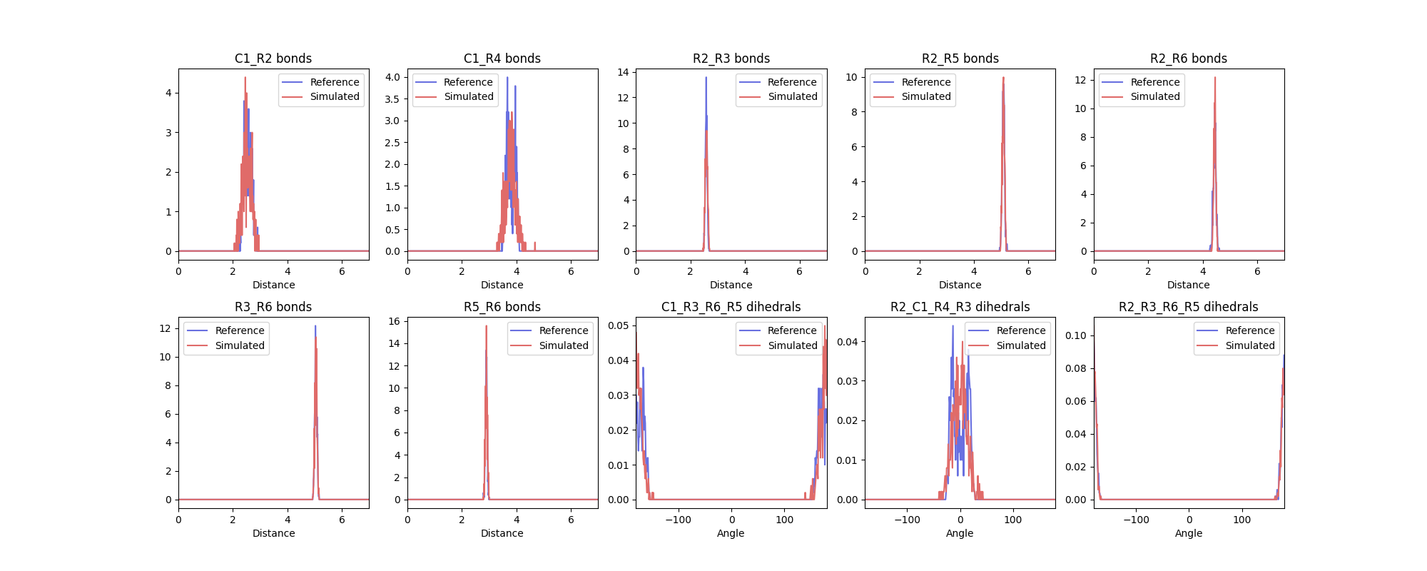
The agreement is very good, noted from both the figure above and also the report of the distribution distance scores generated.
Note that the bimodality of the distributions of the first two dihedrals cannot be captured by the CG model. However, the size of the CG distribution will seemingly capture the two AA configurations into the single CG configuration. If the agreement is not satisfactory at the first iteration - which is likely to happen - you should play with the equilibrium value and force constants in the CG .itp and iterate till satisfactory agreement is achieved.
7. Comparison to experimental results, further refinements, and final considerations
As before it is imperative that any newly parameterised molecule for the Martini force field is validated against as many references as possible.
7.1 Molecular volume and shape
To automate the creation of a vdwradii.dat for a CG molecule, a small Python script, make_cg_sasa_file.py is provided with this tutorial to automate the process. Otherwise, the steps and scripts from the previous tutorial can be followed again.
7.2 Final considerations
This tutorial builds on the Classic Small Molecule Parameterization tutorial using the Fast_Forward package to provide partial automation of some processes. From here, it may be a good idea to explore some of the other features of the package, particularly the ff_inter program, to aid with parameterization of other small molecules from scratch.
Tools and scripts used in this tutorial
GROMACS(http://www.gromacs.org/)Fast_Forward(https://github.com/fgrunewald/fast_forward/tree/main/fast_forward)
References
[1] P.C.T. Souza, et al., Nat. Methods 2021, 18, 382–388.
[2] R. Alessandri, et al., Adv. Theory Simul. 2022, 5, 2100391..
[3] M. Bugnon M, et al., J. Chem. Inf. Model. 2023, 63, 6469-75.
[4] J. Barnoud, https://github.com/jbarnoud/cgbuilder.